Assessing Reliability

Learning Objectives

• Identify the sources of error associated with internal consistency, test-retest, and alternate forms reliability
• Derive the reliability of a composite made up of parallel and tau-equivalent components (i.e., \(\alpha\) coefficient)
• Describe the factors affecting \(\alpha\)
• Explain why high reliability does not imply unidimensionality
• Explain why reliability is a property of test scores, not of the test itself
• Compute reliability for multilevel (longitudinal) test scores

Reliability Coefficients

• Internal consistency
  • Source of random error: item
• Stability
  • Source of random error: time
• Equivalence
  • Source of random error: forms

Parallel Items

For \(k\) items \(X_1\), \(X_2\), \(\ldots\), \(X_k\), treat each item as a “test”

Scenario 1: three parallel “tests”

Variances and Covariances

For any item \(j\), \(X_j\) = \(T\) + \(E_j\)

• \(Var(X_j)\) = \(\sigma^2_X\) = \(\sigma^2_T\) + \(\sigma^2_E\)

For any item \(j\) and \(j'\),

• \(Cov(X_j, X_{j'})\) = \(\sigma_{j j'}\) = \(Cov(T + E_j, T + E_{j'})\) = \(Cov(T, T)\) = \(Var(T)\)

Let \(\mathbf{X} = [X_1, X_2, \ldots, X_k]^\top\)

Covariance Matrix of \(\mathbf{X}\):

\[ Var(\mathbf{X}) = \begin{bmatrix} \sigma^2_X & & & \\ \sigma^2_T & \sigma^2_X & & \\ \vdots & \vdots & \ddots & \\ \sigma^2_T & \sigma^2_T & \cdots & \sigma^2_X \end{bmatrix} \]

      x1    x2    x3
x1 29.20 25.73 25.18
x2 25.73 30.27 25.82
x3 25.18 25.82 29.48

Composite

aka sum score: \(Z\) = \(X_1\) + \(X_2\) + \(\ldots\) + \(X_k\) = \(\sum_{j = 1}^k X_j\)

In matrix form: \(Z = \mathbf{1}^\top \mathbf{X}\), where \(\mathbf{1}^\top\) is a row vector of all ones

\(Var(Z)\) = \(\mathbf{1}^\top Var(\mathbf{X}) \mathbf{1}\)

• i.e., summing every element in the \(Var(\mathbf{X})\) matrix

There are \(k\) elements in the diagonal (\(\sigma^2_X\)), and it can be shown that there are \(k (k - 1)\) elements in the off diagonal (\(\sigma^2_T\))

Reliability of Composite Score of Parallel Items

\[ \begin{aligned} Var(Z) & = k \sigma^2_X + k (k - 1) \sigma^2_T \\ & = k (\sigma^2_T + \sigma^2_E) + k (k - 1) \sigma^2_T \\ & = \underbrace{k^2 \sigma^2_T}_{\text{true score component}} + \underbrace{k \sigma^2_E}_{\text{error component}} \end{aligned} \]

Because reliability = variance due to true score / total variance

\[ \rho_{Z Z'} = \frac{k^2 \sigma^2_T}{k \sigma^2_X + k (k - 1) \sigma^2_T} = \frac{k \sigma^2_T}{\sigma^2_X + (k - 1) \sigma^2_T} \]

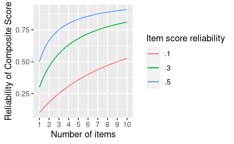
Spearman-Brown Prophecy Formula

For item/test \(X\), its reliability \(\rho_{XX'} = \sigma^2_T / \sigma^2_X\), and \(1 - \rho_{XX'} = \sigma^2_E / \sigma^2_X\), so we have

\[ \rho_{Z Z'} = \frac{k \sigma^2_T / \sigma^2_X}{\sigma^2_X / \sigma^2_X + (k - 1) \sigma^2_T / \sigma^2_X} = \frac{k \rho_{XX'}}{1 + (k - 1) \rho_{XX'}} \]

Important

If \(Z\) is the sum/composite of multiple parallel test scores, and the reliability of each component test score is known, the reliability of \(Z\) can be obtained with the above formula.

Reliability of Composite Score of Essentially Tau-Equivalent Items

Scenario 2: three essentially tau-equivalent “tests”

\(\sigma^2_{X_1}\) = \(\sigma^2_T + \sigma^2_{E_1}\) \(\neq\) \(\sigma^2_{X_2}\)

\(Cov(X_1, X_2)\) = \(\sigma_{12}\) is still \(\sigma^2_T\)

Covariance Matrix of \(\mathbf{X}\):

\[ Var(\mathbf{X}) = \begin{bmatrix} \sigma^2_{X_{\color{red}1}} & & & \\ \sigma^2_T & \sigma^2_{X_{\color{red}2}} & & \\ \vdots & \vdots & \ddots & \\ \sigma^2_T & \sigma^2_T & \cdots & \sigma^2_{X_{\color{red}3}} \end{bmatrix} \]

      x1    x2    x3
x1 29.20 24.17 25.30
x2 24.17 39.68 24.51
x3 25.30 24.51 26.57

Coefficient \(\alpha\)

Total variance: \(\mathbf{1}^\top Var(\mathbf{X}) \mathbf{1}\) = \(\sum_{j \neq j'} \sigma_{jj'}\) + \(\sum_{j = 1}^k \sigma^2_{X_k}\)

\(\sum_{j \neq j'} \sigma_{jj'}\) = \(k (k - 1) \sigma^2_T\) \(\Rightarrow\) \(k \sigma^2_T\) = \(\sum_{j \neq j'} \sigma_{jj'} / (k - 1)\)

\[ \begin{aligned} \rho_{Z Z'} & = \frac{k^2 \sigma^2_T}{ \sum_{j \neq j'} \sigma_{jj'} + \sum_{j = 1}^k \sigma^2_{X_k}} = \frac{k \sum_{j \neq j'} \sigma_{jj'} / (k - 1)}{\sum_{j \neq j'} \sigma_{jj'} + \sum_{j = 1}^k \sigma^2_{X_k}} \\ & = \frac{k}{k - 1} \left(1 - \frac{\sum_{j = 1}^k \sigma^2_{X_k}}{\sum_{j \neq j'} \sigma_{jj'} + \sum_{j = 1}^k \sigma^2_{X_k}}\right) \\ & = \frac{k}{k - 1} \left(1 - \frac{\sum \sigma^2_{X_k}}{\sigma^2_Z}\right) \end{aligned} \]

Exercise

Calculate \(\alpha\) for the following covariance matrix

      x1    x2    x3
x1 29.20 24.17 25.30
x2 24.17 39.68 24.51
x3 25.30 24.51 26.57

Notes on \(\alpha\)

• \(\alpha\) is high when (a) the items are strongly and positively correlated, and/or (b) the number of items is large
  • For (b), it’s because the number of covariances increases as a function of \(k^2\)
• An \(\alpha\) close to 1 with a small number of items could mean that the items are too narrow/similar, and do not cover the full construct domain
• For congeneric items, assuming that errors are truly random, \(\alpha\) is a lower bound to the true reliability value
  • See pp. 177–179 of Bandalos (2018)

\(\alpha\) and Unidimensionality

Unidimensionality: the extent to which a scale measures only one dimension

A high \(\alpha\) does not imply that the items are unidimensional

• It could mean that the number of items is large, and the different dimensions are somewhat positively correlated

Example

data(bfi, package = "psych")
# Agreeableness items
psych::alpha(bfi[1:5], check.keys = TRUE)$total$raw_alpha

[1] 0.7030184

# Conscientiousness items
psych::alpha(bfi[6:10], check.keys = TRUE)$total$raw_alpha

[1] 0.726735

# Agreeableness + Conscientiousness items
psych::alpha(bfi[1:10], check.keys = TRUE)$total$raw_alpha

[1] 0.733409

Computing \(\alpha\) does not require unidimensionality, as long as the overall composite score is meaningful

• E.g., cognitive ability tests usually have multiple dimensions (e.g., verbal, visual-spatial, etc), but the overall score is usually interpreted

Notes on \(\alpha\) (cont’d)

• Be sure to recode negative items before computing \(\alpha\)
• When errors of some items are correlated (e.g., wording similarity), \(\alpha\) could be an overestimate of true reliability
• Recent guidelines generally suggest having \(\alpha\) of at least .80. The requirement is higher when tests are used for making high-stake decisions
• Confidence intervals for \(\alpha\) should be reported (see R note)
• \(\alpha\) may be inflated for highly speeded tests

Alternative Coefficients for Composites

• Greatest lower bound
• Coefficient \(\omega\)

In many applied situations, when unidimensionality holds, the discrepancy between \(\alpha\) and true reliability is small

To get a glimpse of the long debate regarding \(\alpha\), see McNeish (2018), Raykov & Marcoulides (2019), and Savalei & Reise (2019).

KR-20

By Küder and Richardson

Same as \(\alpha\) by for binary items, with \(\sigma^2_{X_j}\) = \(p_j q_j\), where \(p\) is proportion correct and \(q\) is \(1 - p\)

Reliability is a Property of Test Scores

!!! It is Not a property of the test

Say:

• Score reliability in the current sample is \(\alpha\) = .XX; or
• The reliability coefficient estimated from the scores on Test X for our sample was \(\alpha\) = .XX

Do not say:

• The reliability of test X is \(\alpha\) = .XX

Test-Retest Reliability

Correlation between pre and post scores

Instability could be due to

• unstable measure
• non-uniform changes in constructs across participants
  • Particularly likely for mood, etc

Standard Error of Measurement

aka margin of error for test score

SEM = \(\sigma_E\) = \(\sigma_X \sqrt{1 - \rho_{XX'}}\)

E.g., On an IQ test with SD = 15 and a reliability of .84, the SEM is 6. So for a person with a score of 110, the 95% CI is roughly 110 \(\pm\) 12, or [98, 122].

1. It’s \(\sigma\), not \(\sigma^2\)

2. SEM is an average estimate, not specific to a particular individual

Reliability of Difference Scores

Difference score: \(D\) = \(X_2 - X_1\) (Post - Pre)

\[Var(D) = \sigma^2_{X_1} + \sigma^2_{X_2} - 2 \sigma_{X_1, X_2}\]

True score: \(T_2 - T_1\)

\[ \begin{aligned} Var(T_2 - T_1) & = \sigma^2_{T_1} + \sigma^2_{T_2} - 2 \sigma_{T_1, T_2} \\ & = \underbrace{\rho_{X_1 X_1'}}_{\text{reliability at Time 1}} \sigma^2_{X_1} + \underbrace{\rho_{X_2 X_2'}}_{\text{reliability at Time 2}} \sigma^2_{X_2} \\ & \quad - 2 \underbrace{\rho_{X_1 X_2}}_{\text{pre-post correlation}} \sigma_{X_1} \sigma_{X_2} \end{aligned} \]

Exercise

Reliability of \(D\) decreases with larger pre-post correlations

Calculate \(\rho_{D D'}\) with \(\rho_{X_1 X_1'}\) = .80, \(\rho_{X_2 X_2'}\) = .90, \(\sigma^2_{X_1} = 3\), \(\sigma^2_{X_2} = 5\), and

1. \(\rho_{X_1 X_2}\) = 0.1
2. \(\rho_{X_1 X_2}\) = 0.5
3. \(\rho_{X_1 X_2}\) = 0.9

Multilevel Data

E.g., longitudinal data (lv 1: repeated observations; lv 2: people)

E.g., lv 1: participants; lv 2: sites

Three types of composites, so three \(\alpha\) coefficients

• \(\alpha^{2l}\) for Overall (\(Z\))
• \(\alpha^b\) for between (\(Z^b\) at level 2)
  • E.g., studying individual differences in “trait”
• \(\alpha^w\) for Within (\(Z^w\) at level 1)
  • E.g., studying within-person changes, or “state”

See R note

See Lai (2021)

• Also available at https://quantscience.rbind.io/files/Lai_2020_pm_mcfa_reliability_am.pdf