Factor Analysis

Learning Objectives

• Write down the mathematical expression of the common factor model
• Define factors, loadings, and uniqueness
• Describe the differences between exploratory and confirmatory factor analysis
• Be familiar with the major considerations in EFA, including factor extraction and rotation
• Conduct EFA in R, and interpret and report the results

Validity

Internal structure

• Does the test really reflect the number of dimensions we hypothesized?

Or a more bottom-up question

• E.g., how many dimensions are there among questions for moral values?

Dimensionality

How many dimensions are there underlying a set of items?

• Theoretical importance: validating theory/measure
• Practical importance: useful for scoring, research, etc
  • Imagine studying the association between every item and the outcome

Factor Analysis

Factor: unobserved, latent variables hypothesized to explain the covariance of multiple items

• How many factors are there?
• What do these factors represent?
• Are these factors consistent with my theory?

Common Factor Model

\(j\) indexes item. \(Z_j\) is the \(z\)-score for item \(j\)

\[Z_j = \lambda_{j1} F_1 + \lambda_{j2} F_2 + \cdots + U_j\]

• \(\lambda\) = (standardized) loading
• \(U\) = unique factor; Var(\(U\)) = uniqueness

Common Factor Model (Matrix form)

\[ \begin{bmatrix} Z_1 \\ Z_2 \\ \vdots \\ Z_p \end{bmatrix} = \begin{bmatrix} \lambda_{11} & \lambda_{12} & \ldots \\ \lambda_{21} & \lambda_{22} & \ldots \\ \vdots & \vdots & \ddots \\ \lambda_{p1} & \lambda_{p2} & \ldots \\ \end{bmatrix} \begin{bmatrix} F_1 \\ F_2 \\ \vdots \end{bmatrix} + \begin{bmatrix} U_1 \\ U_2 \\ \vdots \\ U_p \\ \end{bmatrix} \]

\[\mathbf{Z} = \boldsymbol{\Lambda} \mathbf{F} + \mathbf{U}\]

Corr(\(\mathbf{F}\)) = \(\boldsymbol{\Psi}\)

Cov(\(\mathbf{U}\)) = \(\boldsymbol{\Theta}\)

Diagram

Assumptions

• Causal direction: from factors to items
• Realist vs. constructivist (e.g., Borsboom et al., 2003) ¹

• Local independence (\(\boldsymbol{\Theta}\) is diagonal)
  • Observed variables are not dependent (associated) after accounting for the latent variables
  • In other words, observed variables are related just because of the latent variables

1. https://doi.org/10.1037/0033-295X.110.2.203

Path-Tracing

Corr(\(x_1\), \(x_2\)) = a * b

Corr(\(x_2\), \(x_5\)) = b * r * f

Corr(\(x_3\), \(x_4\)) = c * d + c * r * e

Vanishing Tetrad

Because latent variables are not observed, we can only test the implication of local independence, which is called vanishing tetrad

• For unidimensional test, it requires four items (thus, tetrad)

Let \(Q_{ij}\) = Corr(\(x_i\), \(x_j\)). If local independence holds,

• \(Q_{12}Q_{34}\) = ab * cd
• \(Q_{13}Q_{24}\) = ac * bd

So this implies

• \(Q_{12}Q_{34}\) - \(Q_{13}Q_{24}\) = 0
• \(Q_{12}Q_{34}\) - \(Q_{14}Q_{23}\) = 0
• \(Q_{13}Q_{24}\) - \(Q_{14}Q_{23}\) = 0

Exercise

Are the items unidimensional?

\[ \begin{bmatrix} 1 & & & \\ 0.5 & 1 & & \\ 0.5 & 0.4 & 1 & \\ 0.3 & 0.5 & 0.5 & 1 \\ \end{bmatrix} \]

Note on Model Fit

In practice, an overall test is more commonly used to assess local independence

• Nevertheless, it helps to know what the overall test is actually testing, i.e., a set of vanishing tetrad assumptions.

Model fit shows whether the assumptions (i.e., local independence) are tenable

A good fit does not confirm the factor model, as alternative models may have the same implications on the data

Exploratory vs. Confirmatory

In practice, the distinction is usually blurred

	EFA	CFA
Goal	Explore number of factors and factor structure	Test theory-driven model
Matrix analyzed	Usually correlation matrix	Usually covariance matrix
Loading structure	No restriction	Usually simple structure with few cross-loadings
Identification	Assume uncorrelated factors initially; use rotation to find interpretable solution	Use reference indicator or standardized factors

Exploratory vs. Confirmatory (cont’d)

	EFA	CFA
Local independence	Required	Usually assumed, but can be relaxed
Usual estimation method	PAF, ML, ULS	ML and WLS
Model evaluation	Correlation residuals, proportion of variance accounted for, interpretability	Global chi-squared test and goodness-of-fit indices, correlation residuals

Steps of EFA

• Obtain correlation matrix (Pearson, polychoric, etc)
• Factor extraction
• Determining number of factors
• Rotating the factors
• Interpreting the factors
• Replicating or confirming of the results

Correlation Matrix

	y1	y2	y3
y1	1	.	.
y2	.61	1	.
y3	.44	.55	1

library(plotly)
plot_ly(dfy, x = ~ y1, y = ~ y2, z = ~ y3,
        size = 5,
        width = 480, height = 480)

If items are ordinal, use polychoric correlation

Extraction

Component Analysis

• Based on full correlation matrix

1.0	0.5	0.5	0.3
0.5	1.0	0.4	0.5
0.5	0.4	1.0	0.5
0.3	0.5	0.5	1.0

Component = linear combinations of items; no uniqueness

Useful for forming composites; usually not theoretically driven

Factor Analysis

• Diagonals are communalities

0.36	0.50	0.50	0.30
0.50	0.38	0.40	0.50
0.50	0.40	0.38	0.50
0.30	0.50	0.50	0.36

Factor = common cause of items; each item has uniqueness

Useful for theory-driven measurement models

Communalities

Common/shared variance of an item with other items
= 1 - uniqueness

Can be estimated using

• \(R^2\) of all other variables predicting \(X_j\)
  • Equivalent to the diagonal of the inverse of the correlation matrix, \([Corr(\mathbf{X})]^{-1}\)
• Iterative methods
  • Initial communalities, find loadings, compute communalities again, until convergence (i.e., changes are minimal)

Extraction Methods

• Principal axis factoring (PAF)
  • Based on eigen-decomposition
• Maximum likelihood (ML)
  • Assume normal distribution
• Unweighted least squares (ULS)
  • Minimize sum of squared differences in elements of observed and implied correlation matrices

There are many more extraction methods. See e.g., the documentation of the fm option in the psych::fa() function in R.

Eigen Decomposition of Symmetric Matrix R

\[\mathbf{R} = \mathbf{Q} \mathbf{D} \mathbf{Q}^\top\]

where \(\mathbf{D}\) is a diagonal matrix of eigenvalues, and \(\mathbf{Q}\) is an orthogonal values of eigenvectors

eigen_r <- eigen(rr_mat)
eigen_r$values # eigenvalues; sum to p

[1]  1.72549364  0.06222222 -0.01500000 -0.27827141

eigen_r$vectors # unscaled loadings

           [,1]          [,2]          [,3]       [,4]
[1,] -0.4844395 -7.071068e-01  0.000000e+00  0.5150907
[2,] -0.5150907  5.551115e-17 -7.071068e-01 -0.4844395
[3,] -0.5150907 -1.387779e-16  7.071068e-01 -0.4844395
[4,] -0.4844395  7.071068e-01  5.551115e-17  0.5150907

# Get back the correlation
eigen_r$vectors %*% diag(eigen_r$values) %*% t(eigen_r$vectors)

          [,1]  [,2]  [,3]      [,4]
[1,] 0.3622222 0.500 0.500 0.3000000
[2,] 0.5000000 0.385 0.400 0.5000000
[3,] 0.5000000 0.400 0.385 0.5000000
[4,] 0.3000000 0.500 0.500 0.3622222

To convert eigenvectors to loadings, multiply by the square root of the corresponding eigenvalue

# Just the first two factors
(lambda <- 
    sweep(eigen_r$vectors[, 1:2], MARGIN = 2,
          STATS = sqrt(eigen_r$values[1:2]), FUN = "*"))

           [,1]          [,2]
[1,] -0.6363502 -1.763834e-01
[2,] -0.6766130  1.384691e-17
[3,] -0.6766130 -3.461728e-17
[4,] -0.6363502  1.763834e-01

# Recompute communalities
rowSums(lambda^2)

[1] 0.4360527 0.4578052 0.4578052 0.4360527

# Then repeat the process

In initial factor extraction, \(\boldsymbol{\Psi}\) is an identity matrix, meaning that the factors are uncorrelated.

Find more information on Wikipedia: https://en.wikipedia.org/wiki/Eigendecomposition_of_a_matrix

Number of Factors

We can extract as many as \(p\) factors, where \(p\) is the number of items, but this is not very useful

• Each factor just explain one item

Sometimes there are nuisance factors based on wording similarities, and we usually don’t want to extract those

Some methods for determining number of factors

• K1 rule (not recommended)
• Scree plot (subjective)
  • See Figure 12.4 and discussion in text
• Parallel analysis (recommended)
• The Hull method (recommended)
  • Generalization of scree test; see text and the EFAtools R package

K1 Rule

If there is no common factor, items are uncorrelated, and all eigenvalues will be close to 1

So historically, researchers used number of eigenvalues > 1 as the number of factors

• This is not recommended any more, but still the default in some software (e.g., SPSS)

Parallel Analysis

Improve K1 by taking into account the random noise in sample eigenvalues

1. Generate random data sets when there are no factors (i.e., items are uncorrelated)
   • Need to know the sample size (\(N\))
2. For each data set, obtain eigenvalues based on full or reduced correlation matrix ¹
3. Retain factors when the \(k\)th sample eigenvalue is larger than the average (or 95%) of the \(k\)th sample eigenvalues from the random data

1. My experience is that using the full matrix is a bit more reliable even for factor analysis, mainly because using \(R^2\) for communalities may not be very reliable. See more discussion in, e.g., https://doi.org/10.1037/met0000230 and http://doi.org/10.1037/met0000269.

E.g., eigenvalues for a random data set

# Example with one simulated data
set.seed(1314)
num_var <- 4
num_obs <- 100
random_r <- cor(
    matrix(rnorm(num_var * num_obs), nrow = 100, ncol = 4)
)
# Eigenvalues
eigen(random_r)$values

[1] 1.1962797 1.1648113 0.8617416 0.7771674

Remarks on Factor Extraction

• Statistical criterion is only suggestive; interpretability and theoretical relevance is also important.

• One should routinely examine multiple criteria, such as with parallel analysis AND the psych::nfactors() function.

• Other considerations: loading pattern, correlation residual (model fit).

• If the software suggested \(k\) factors, \(k \pm 1\) factors may still be reasonable.

Rotation

Factor Indeterminacy:

\[Corr(\boldsymbol{X}) = \boldsymbol{\Lambda} \boldsymbol{\Psi} \boldsymbol{\Lambda}^\top + \boldsymbol{\Theta}\]

We can define arbitrary transformation of \(\boldsymbol{\Lambda}*\) = \(\boldsymbol{\Lambda} \mathbf{T}\) and \(\boldsymbol{\Psi}*\) = \(\mathbf{T}^{-1} \boldsymbol{\Psi} {\mathbf{T}^\top}^{-1}\), and get exactly the same implied correlation.

Therefore, there are infinitely many choices of loading matrix, the goal of rotation is to choose the most interpretable solution.

Rotation DOES NOT change model fit

Variable and Factor Complexity

Sum of cross-products of squared loadings

• Squared loadings are closer to zero when the original values are small to moderate
  • E.g., .9^2 = .81; .5^2 = .25; .1^2 = .01
• Cross product will be small if one of the loading is small
  • E.g., .5^2 * .5^2 = .0625, but .9^2 * .1^2 = .0081

Low variable complexity: each item has high loading on only one factor (i.e., cross-loadings are small)

Low factor complexity: each factor has only a few items with strong loadings on it

Most rotation methods find a solution that minimizes a weighted sum of variable and factor complexity

Simple Structure (see p. 332 of text)

• Sometimes minimizing cross-loadings may lead to problems (more on this in CFA)

Some Common Rotation Methods

Orthogonal rotations (uncorrelated factors)

• Varimax, Quartimax, etc

Oblique rotations (correlated factors)

• Oblimin, promax (m = 2 to 4), etc

One should “choose the most interpretable and theoretically defensible result” (Bandalos, 2018, p. 334)

Unrotated

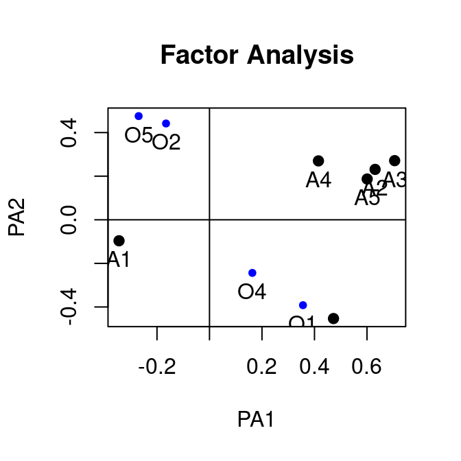
Oblimin

Target Rotation

Often researchers have some ideas of which items may (or may not) load on some factors. Such information can be coded in target rotation by specifying a target matrix.

E.g., First five items on factor 1, next five items on factor 2

      [,1] [,2]
 [1,]   NA    0
 [2,]   NA    0
 [3,]   NA    0
 [4,]   NA    0
 [5,]   NA    0
 [6,]    0   NA
 [7,]    0   NA
 [8,]    0   NA
 [9,]    0   NA
[10,]    0   NA

Then the rotation algorithm will try to get the cross-loadings to zero.

Correlation Residual

Let \(r_{jj'}\) be sample correlation between item \(j\) and \(j'\), then correlation residual is

\[r_{jj'} - \hat{\boldsymbol{\Sigma}}_{jj'}\]

where \(\hat{\boldsymbol{\Sigma}}\) is the implied correlation matrix based on EFA with \(q < p\) factors.

Rule of thumb

If there is a cluster of variables with correlation residual > .10 in absolute values, it may suggest underfactoring.

Reporting

See the text for an example with justification of different decisions

See https://doi.org/10.1177/0095798418771807 for information to include (Table 1) and an example report

Sample APA table: https://apastyle.apa.org/style-grammar-guidelines/tables-figures/sample-tables#factor

Replicating Factor Structure

By definition, EFA is exploratory, which means that its result requires some validation.

• Replication should be done in an independent sample
• Avoid dropping items until low loadings are replicated on an independent sample

Data and Sample Size Requirements

• KMO and Bartlett’s test
  • Is there evidence for any factor?
• If discrete/skewed, use the right correlation
  • E.g., tetrachoric/polychoric for binary/ordinal
  • Robust correlation
• Needs larger \(N\) with low communality level and variable-factor ratio
  • For \(q = 3\) factors, Bandalos suggested
    • \(N\) = 100/300 if average communality = .7/.5; \(N\) = 500 otherwise