        I1    I2    I3    I4     I5    I6     I7    I8    I9   I10    I11   I12
I1   1.000 0.690 0.702 0.166  0.163 0.293 -0.040 0.143 0.078 0.280  0.182 0.112
I2   0.690 1.000 0.712 0.245  0.248 0.421  0.068 0.212 0.145 0.254  0.202 0.154
I3   0.702 0.712 1.000 0.188  0.179 0.416  0.021 0.217 0.163 0.223  0.186 0.128
I4   0.166 0.245 0.188 1.000  0.380 0.482  0.227 0.218 0.119 0.039  0.012 0.029
I5   0.163 0.248 0.179 0.380  1.000 0.377  0.328 0.280 0.254 0.066 -0.008 0.021
I6   0.293 0.421 0.416 0.482  0.377 1.000  0.238 0.325 0.301 0.059  0.051 0.084
I7  -0.040 0.068 0.021 0.227  0.328 0.238  1.000 0.386 0.335 0.018  0.052 0.160
I8   0.143 0.212 0.217 0.218  0.280 0.325  0.386 1.000 0.651 0.152  0.202 0.221
I9   0.078 0.145 0.163 0.119  0.254 0.301  0.335 0.651 1.000 0.129  0.177 0.205
I10  0.280 0.254 0.223 0.039  0.066 0.059  0.018 0.152 0.129 1.000  0.558 0.483
I11  0.182 0.202 0.186 0.012 -0.008 0.051  0.052 0.202 0.177 0.558  1.000 0.580
I12 0.112 0.154 0.128 0.029 0.021 0.084 0.160 0.221 0.205 0.483 0.580 1.000Factor Analysis
Learning Objectives
- Explain the differences between EFA and CFA
- Compute the degrees of freedom for a CFA model with covariance matrix as input
- Explain the need for identification constraints to set the metrics of latent factors
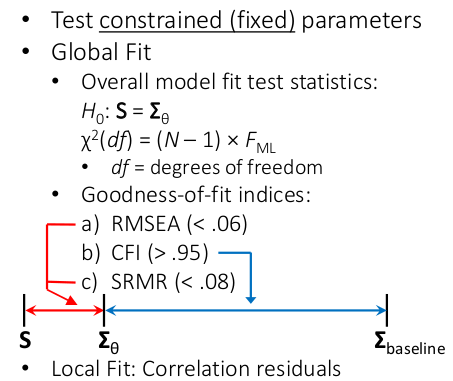
- Explain the pros and cons of the global \(\chi^2\) test and the goodness-of-fit indices
- Run a CFA in R and interpret the model fit and the parameter estimates
- Write up the result section reporting CFA results
From EFA to CFA
- CFA requires specifying the zeros in the \(\boldsymbol \Lambda\) matrix
- Flexibility in specifying unique covariances (i.e., off-diagonal elements in \(\boldsymbol \Theta\))
- Analyze items in original metric (not \(z\)-scores)
- The covariance matrix, \(\boldsymbol \Sigma = \text{Cov}(\mathbf{X})\) is analyzed
- Results are usually unstandardized, and not comparable to standardized coefficients (as in EFA)
Notation
\[\boldsymbol \Sigma = \boldsymbol \Lambda \boldsymbol \Psi \boldsymbol \Lambda^\top + \boldsymbol \Theta\]
\(\boldsymbol \Psi = \begin{bmatrix} \psi_{11} & \psi_{12} & \ldots \\ \psi_{12} & \psi_{22} & \ldots \\ \vdots & \vdots & \ddots \\ \psi_{1q} & \psi_{2q} & \ldots \\ \end{bmatrix}\), \(\boldsymbol \Theta = \begin{bmatrix} \theta_{11} & \theta_{12} & \ldots \\ \theta_{12} & \theta_{22} & \ldots \\ \vdots & \vdots & \ddots \\ \theta_{1q} & \theta_{2q} & \ldots \\ \end{bmatrix}\)
Implied Variances and Covariances
Implied variance of item \(i\): \(\sum_k^q \lambda_{ik}^2 \psi_{kk} + \sum_k^q \sum_{l \neq k} \lambda_{ik} \lambda_{il} \psi_{kl} + \theta_{ii}\)
Implied covariance between item \(i\) and \(j\): \(\sum_k^q \sum_l^q \lambda_{iq} \psi_{kl} \lambda_{jl} + \theta_{ij}\)
See Table 13.2 of text
Steps for CFA
- Data preparation
- Model specification
- Model identification
- Estimation of parameters
- Model evaluation
- Model modification
Data Input
- Raw data; (2) covariance matrix; (3) correlation matrix and SDs
Achievement Goal Questionnaire (p. 358 of text)
Correlation
Covariance
sds <- c(1.55, 1.53, 1.56, 1.94, 1.68, 1.72, # typo in Table 13.3
         1.42, 1.50, 1.61, 1.18, 0.98, 1.20)
covy <- diag(sds) %*% cory %*% diag(sds)
I1 I2 I3 I4 I5 I6 I7 I8 I9 I10 I11 I12
I1 2.403 1.636 1.697 0.499 0.424 0.781 -0.088 0.332 0.195 0.512 0.276 0.208
I2 1.636 2.341 1.699 0.727 0.637 1.108 0.148 0.487 0.357 0.459 0.303 0.283
I3 1.697 1.699 2.434 0.569 0.469 1.116 0.047 0.508 0.409 0.410 0.284 0.240
I4 0.499 0.727 0.569 3.764 1.238 1.608 0.625 0.634 0.372 0.089 0.023 0.068
I5 0.424 0.637 0.469 1.238 2.822 1.089 0.782 0.706 0.687 0.131 -0.013 0.042
I6 0.781 1.108 1.116 1.608 1.089 2.958 0.581 0.839 0.834 0.120 0.086 0.173
I7 -0.088 0.148 0.047 0.625 0.782 0.581 2.016 0.822 0.766 0.030 0.072 0.273
I8 0.332 0.487 0.508 0.634 0.706 0.839 0.822 2.250 1.572 0.269 0.297 0.398
I9 0.195 0.357 0.409 0.372 0.687 0.834 0.766 1.572 2.592 0.245 0.279 0.396
I10 0.512 0.459 0.410 0.089 0.131 0.120 0.030 0.269 0.245 1.392 0.645 0.684
I11 0.276 0.303 0.284 0.023 -0.013 0.086 0.072 0.297 0.279 0.645 0.960 0.682
I12 0.208 0.283 0.240 0.068 0.042 0.173 0.273 0.398 0.396 0.684 0.682 1.440Exercise
Draw a path diagram with Items 1-3 loaded on one factor, Items 4-6 loaded on the second, Items 7-9, and Items 10-12 loaded on the fourth.
Write out the \(\boldsymbol{\Lambda}\) matrix
Figure 13.2
Curved double-headed arrows indicate variances/covariances
Model Identification
A set of parameters is not identified when multiple set of values leads to the same estimation criterion
E.g., \(5 = a + b\): \(a = 2, b = 3\); \(a = 10, b = -5\), etc
In CFA, as we are fitting the covariance matrix, we can have at most \(p \times (p + 1) / 2\) parameters, which will perfectly reproduce the variances and covariances
- Underidentified: # parameters > \(p \times (p + 1) / 2\)
- Just-identified: # parameters = \(p \times (p + 1) / 2\)
- Overidentified: # parameters < \(p \times (p + 1) / 2\)
Degrees of freedom (df): \(p \times (p + 1) / 2\) \(-\) # parameters
Exercise
For a one-factor model with three items, is it underidentified, just-identified, or overidentified?
Setting the Factor Metric
E.g., is IQ (latent factor) measured as \(z\)-scores? \(T\) scores? other choices?
Important
Latent factors do not have intrinsic units. This needs to be set for each latent variable.
The choice is usually arbitrary, but the common options are
- Standardizing the latent factors (i.e., they are in \(z\)-scores)
- Setting the loading of the first item (called reference indicator) to 1
Additional Notes
Having (a) df ≥ 0 and (b) set the metric for each latent variable are only necessary, but not sufficient, conditions for identification
Tip
Generally speaking, we need three indicators per factor for identification.
Estimation
Find values for the free elements in \(\boldsymbol \Lambda\), \(\boldsymbol \Psi\), and \(\boldsymbol \Theta\) that minimize the discrepancy between
- \(\boldsymbol S\): the input covariance matrix, and
- \(\hat{\boldsymbol \Sigma}\): the implied covariance matrix
Common estimation methods
- Maximum likelihood (ML) based on normal distributions
- Typically used for continuous data
- Also for items with 5 and more categories (with small to moderate skewness)
- Use adjusted standard errors (
estimator = "mlm"orestimator = "mlr")
- Use adjusted standard errors (
- Weighted least squares (WLS)
- Includes ULS as a special case
- Fast approximation for discrete items (5 or fewer categories)
Maximum Likelihood
Log-likelihood function: \(\ell(\boldsymbol\Sigma; \mathbf S) = - \frac{Np}{2} \log(2\pi) - \frac{N}{2} \log |\boldsymbol \Sigma| - \frac{N - 1}{2} \mathrm{tr} \left(\boldsymbol \Sigma^{-1} \mathbf S\right)\)
Discrepancy function: \(\log |\hat{\boldsymbol \Sigma}| - \log |\tilde{\mathbf S}| + \mathrm{tr} \left(\hat{\boldsymbol \Sigma}^{-1}\tilde{\mathbf S}\right) - p\)
Model \(\chi^2\) Test
Null hypothesis: \(\boldsymbol \Sigma = \boldsymbol \Sigma_0\)
- i.e., the model-implied covariance matrix perfectly fits the population covariance matrix
Important
- Traditional hypothesis testing: aim to support \(H_1\) (rejecting is usually good)
- Goodness-of-fit testing: aim to identify model misfits (rejecting is usually bad)
The model \(\chi^2\) is a likelihood ratio test by comparing two models:
- Best model (H1): \(\boldsymbol \Sigma = \boldsymbol S\), df1 = 0
- Hypothesized model (H0): \(\boldsymbol \Sigma = \hat{\boldsymbol \Sigma}\), df0 > 0
Under the null, in large samples, the test statistic T follows a chi-squared distribution, with df = df0
Model Test User Model:

  Test statistic                               284.046
  Degrees of freedom                                48
  P-value (Chi-square)                           0.000
Missing Data
- Full information maximum likelihood (FIML)
missing = "fiml"in lavaan- Useful for ignorable missingness (i.e., missing [completely] at random)
- Cause of missingness can be explained by observed values in the data
- Multiple imputation
- More flexible, but more tedious specifications
Non-normality
If univariate |skewness| or |kurtosis| > 2.0, or normalized multivariate kurtosis > 3.0
 [1]  0.82504356 -1.12428533 -0.99845684 -1.03094275 -0.84723335 -0.85470158
 [7] -0.74181968 -0.69145540  0.59617294  0.06616716  0.37345508  0.22082058
[13] -0.47037917 -0.82374021 -0.77706636  0.37122930 -0.07694366  0.15059864
[19]  0.19688969  0.37425725 -0.89688239  0.58536528 -0.77263334 -1.21759120
[25] 0.73808342 A1 A2 A3 A4 A5 C1
-0.30763947 1.05483862 0.44204096 0.04045252 0.15890562 0.30442934
C2 C3 C4 C5 E1 E2
-0.13643987 -0.13233095 -0.62141881 -1.21666936 -1.09233560 -1.14863822
E3 E4 E5 N1 N2 N3
-0.46511252 -0.30422493 -0.09369184 -1.01285920 -1.05105088 -1.17860226
N4 N5 O1 O2 O3 O4
-1.09235018 -1.06128795 0.42523597 -0.81267459 0.30198047 1.07975589
O5
-0.23897800 Call: psych::mardia(x = bfi[1:25])
Mardia tests of multivariate skew and kurtosis
Use describe(x) the to get univariate tests
n.obs = 2436 num.vars = 25
b1p = 27.66 skew = 11229.18 with probability <= 0
small sample skew = 11244.07 with probability <= 0
b2p = 781.5 kurtosis = 71.53 with probability <= 0
- Continuous: normal-distribution-based MLM
- Adjust the test statistic for nonnormality in data
- Sandwich estimator for standard errors
- MLR: accounts for missing data
- Categorical: WLSMV
- Diagonal matrix as weight matrix for estimates
- Full weight matrix for standard errors and adjusted test statistic
ac_mod <- "
Ag =~ A1 + A2 + A3 + A4 + A5
Co =~ C1 + C2 + C3 + C4 + C5
"
cfa_ac_wls <- cfa(
    ac_mod,
    data = bfi,
    ordered = TRUE,
    estimator = "WLSMV"  # default
)
cfa_ac_wls
lavaan 0.6.15 ended normally after 25 iterations
Estimator DWLS
Optimization method NLMINB
Number of model parameters 61
Used Total
Number of observations 2632 2800
Model Test User Model:
Standard Scaled
Test Statistic 449.278 593.496
Degrees of freedom 34 34
P-value (Chi-square) 0.000 0.000
Scaling correction factor 0.764
Shift parameter 5.648
simple second-order correction Alternative Fit Indices
How good is the fit, if not perfect?
- RMSEA, CFI: based on \(\chi^2\)
- SRMR: overall discrepancy between model-implied and sample covariance matrix
Danger
Good model fit does not mean that the model is useful. Pay attention to the parameter values
lavaan 0.6.15 ended normally after 46 iterations

  Estimator                                         ML
  Optimization method                           NLMINB
  Number of model parameters                        30

  Number of observations                          1022

Model Test User Model:

  Test statistic                               284.046
  Degrees of freedom                                48
  P-value (Chi-square)                           0.000

Model Test Baseline Model:

  Test statistic                              4417.935
  Degrees of freedom                                66
  P-value                                        0.000

User Model versus Baseline Model:

  Comparative Fit Index (CFI)                    0.946
  Tucker-Lewis Index (TLI)                       0.925

Loglikelihood and Information Criteria:

  Loglikelihood user model (H0)             -20021.587
  Loglikelihood unrestricted model (H1)     -19879.564

  Akaike (AIC)                               40103.175
  Bayesian (BIC)                             40251.060
  Sample-size adjusted Bayesian (SABIC)      40155.777

Root Mean Square Error of Approximation:

  RMSEA                                          0.069
  90 Percent confidence interval - lower         0.062
  90 Percent confidence interval - upper         0.077
  P-value H_0: RMSEA <= 0.050                    0.000
  P-value H_0: RMSEA >= 0.080                    0.013

Standardized Root Mean Square Residual:

  SRMR                                           0.050

Parameter Estimates:

  Standard errors                             Standard
  Information                                 Expected
  Information saturated (h1) model          Structured

Latent Variables:
                   Estimate  Std.Err  z-value  P(>|z|)
  PerfAppr =~
    I1                1.000
    I2                1.034    0.036   29.060    0.000
    I3                1.053    0.036   29.039    0.000
  PerfAvoi =~
    I4                1.000
    I5                0.772    0.061   12.678    0.000
    I6                1.197    0.081   14.828    0.000
  MastAvoi =~
    I7                1.000
    I8                1.955    0.149   13.138    0.000
    I9                1.856    0.140   13.303    0.000
  MastAppr =~
    I10               1.000
    I11               0.974    0.052   18.567    0.000
    I12               1.043    0.057   18.196    0.000

Covariances:
                   Estimate  Std.Err  z-value  P(>|z|)
  PerfAppr ~~
    PerfAvoi          0.752    0.074   10.167    0.000
    MastAvoi          0.196    0.034    5.762    0.000
    MastAppr          0.309    0.042    7.396    0.000
  PerfAvoi ~~
    MastAvoi          0.377    0.046    8.275    0.000
    MastAppr          0.080    0.039    2.064    0.039
  MastAvoi ~~
    MastAppr          0.159    0.025    6.457    0.000

Variances:
                   Estimate  Std.Err  z-value  P(>|z|)
   .I1                0.820    0.050   16.300    0.000
   .I2                0.649    0.046   13.968    0.000
   .I3                0.679    0.048   14.026    0.000
   .I4                2.450    0.133   18.465    0.000
   .I5                2.039    0.103   19.751    0.000
   .I6                1.077    0.109    9.890    0.000
   .I7                1.585    0.075   21.188    0.000
   .I8                0.607    0.080    7.637    0.000
   .I9                1.111    0.084   13.208    0.000
   .I10               0.726    0.043   16.785    0.000
   .I11               0.329    0.030   10.846    0.000
   .I12               0.716    0.045   16.088    0.000
    PerfAppr          1.581    0.106   14.955    0.000
    PerfAvoi          1.311    0.148    8.881    0.000
    MastAvoi          0.429    0.061    7.055    0.000
    MastAppr          0.664    0.060   11.084    0.000
For MLR, WLSMV, etc, use the “robust” versions of CFI, RMSEA
Correlation Residuals
$type
[1] "cor.bollen"

$cov
        I1     I2     I3     I4     I5     I6     I7     I8     I9    I10
I1   0.000
I2   0.000  0.000
I3   0.013 -0.010  0.000
I4  -0.084 -0.017 -0.074  0.000
I5  -0.060  0.014 -0.055  0.069  0.000
I6  -0.045  0.067  0.062  0.011 -0.043  0.000
I7  -0.129 -0.025 -0.072  0.090  0.206  0.053  0.000
I8  -0.023  0.039  0.044 -0.036  0.054 -0.017 -0.008  0.000
I9  -0.068 -0.008  0.010 -0.105  0.054 -0.002 -0.014  0.005  0.000
I10  0.111  0.077  0.046  0.004  0.035  0.012 -0.077 -0.024 -0.026  0.000
I11 -0.017 -0.006 -0.022 -0.029 -0.045 -0.004 -0.060 -0.004 -0.005 -0.002
I12 -0.062 -0.027 -0.053 -0.007 -0.011  0.035  0.063  0.041  0.046 -0.007
       I11    I12
I1
I2
I3
I4
I5
I6
I7
I8
I9
I10
I11  0.000
I12  0.006  0.000
Modification Indices
         lhs op rhs     mi    epc sepc.lv sepc.all sepc.nox
110       I5 ~~  I7 40.324  0.384   0.384    0.214    0.214
109       I5 ~~  I6 33.988 -0.594  -0.594   -0.401   -0.401
44  PerfAvoi =~  I1 30.762 -0.236  -0.270   -0.175   -0.175
105       I4 ~~  I9 22.889 -0.309  -0.309   -0.188   -0.188
37  PerfAppr =~  I6 22.686  0.326   0.410    0.238    0.238
41  PerfAppr =~ I10 20.180  0.126   0.159    0.134    0.134
82        I2 ~~  I3 19.945 -0.366  -0.366   -0.551   -0.551
79        I1 ~~ I10 19.607  0.135   0.135    0.175    0.175
72        I1 ~~  I3 17.535  0.312   0.312    0.419    0.419
101       I4 ~~  I5 17.473  0.379   0.379    0.170    0.170
126       I7 ~~ I12 17.032  0.158   0.158    0.148    0.148
53  MastAvoi =~  I1 16.139 -0.235  -0.154   -0.100   -0.100
94        I3 ~~  I6 15.821  0.173   0.173    0.202    0.202
45  PerfAvoi =~  I2 15.410  0.162   0.185    0.121    0.121
57  MastAvoi =~  I5 15.059  0.407   0.267    0.159    0.159
76        I1 ~~  I7 13.676 -0.154  -0.154   -0.135   -0.135
47  PerfAvoi =~  I7 13.051  0.184   0.211    0.149    0.149
35  PerfAppr =~  I4 12.889 -0.228  -0.287   -0.148   -0.148
127       I8 ~~  I9 12.707  0.647   0.647    0.788    0.788
75        I1 ~~  I6 12.595 -0.158  -0.158   -0.169   -0.169
103       I4 ~~  I7 11.602  0.231   0.231    0.117    0.117
92        I3 ~~  I4 10.642 -0.171  -0.171   -0.133   -0.133
Note
- Do modifications in sequential order
- There are usually multiple ways to improve model fit
- E.g., unique covariance vs. cross-loadings
- Modifications should be theoretically justified; otherwise they are usually not replicable
- They could provide insights into the measure and the constructs
- If making too many modifications (e.g., > 3), reconsider your original model
Composite Reliability
If each item only loads on one factor, the omega coefficient is
\[ \small \omega = \frac{(\sum \lambda_i)^2}{(\sum \lambda_i)^2 + \mathbf{1}^\top \boldsymbol{\Theta}\mathbf{1}} \]
Exercise
Compute \(\omega\) for the PerfAvoi factor, using results from the previous slide.
Difference test
- Requires nested models
- Get M0 by placing constraints on M1
- Difference of two \(\chi^2\) test statistic is also a \(\chi^2\), with df = difference in the dfs of the two models
- Need adjustment for MLR, WLSMV, etc
- If constraining parameter on the boundary, need adjusting critical values
- E.g., compare 1- vs. 2-factor by setting factor cor to 1
Example: Parallel Test
# Treat items as continuous for illustrative purposes
ag_congeneric <- "
    Ag =~ A1 + A2 + A3 + A4 + A5
    # Intercepts (default)
    A1 + A2 + A3 + A4 + A5 ~ NA * 1
    # Fixed factor mean
    Ag ~ 0
    # Free variances (default)
    A1 ~~ NA * A1
    A2 ~~ NA * A2
    A3 ~~ NA * A3
    A4 ~~ NA * A4
    A5 ~~ NA * A5
"
con_fit <- cfa(ag_congeneric, data = bfi, estimator = "MLR",
               meanstructure = TRUE)
ag_parallel <- "
# Loadings = 1
Ag =~ 1 * A1 + 1 * A2 + 1 * A3 + 1 * A4 + 1 * A5
# Intercepts = 0
A1 + A2 + A3 + A4 + A5 ~ 0
# Free factor mean
Ag ~ NA * 1
# Equal variances (use same labels)
A1 ~~ v * A1
A2 ~~ v * A2
A3 ~~ v * A3
A4 ~~ v * A4
A5 ~~ v * A5
"
par_fit <- cfa(ag_parallel, data = bfi, estimator = "MLR",
meanstructure = TRUE)
Scaled Chi-Squared Difference Test (method = "satorra.bentler.2001")

lavaan NOTE:
    The "Chisq" column contains standard test statistics, not the
    robust test that should be reported per model. A robust difference
    test is a function of two standard (not robust) statistics.

        Df   AIC   BIC    Chisq Chisq diff Df diff Pr(>Chisq)
con_fit  5 43585 43674   86.696
par_fit 17 51304 51322 7829.963     5837.2      12  < 2.2e-16 ***
---
Signif. codes:  0 '***' 0.001 '**' 0.01 '*' 0.05 '.' 0.1 ' ' 1