Item Response Theory

Learning Objectives

• Explain the meaning of item difficulty and item discrimination in one- and two-parameter IRT models
• Estimate item and person parameters from a Rasch model and a 2PL model in R
• Assess model fit

Factor Analysis and IRT

Both can be formulated as a latent variable model

Discrete Response Options

Some basic IRT models

• Binary/dichotomous: Rasch, 1PL, 2PL, 3PL (and the Normal ogive models)
• Polytomous: rating scale, graded response, (generalized) partial credit

Note

The underlying mathematical model of (a) factor analysis with ordinal items (sometimes called item factor analysis) and (b) the basic IRT is the same. However, they are usually estimated with different estimators, and they have different traditions in the analytic procedures and statistics computed.

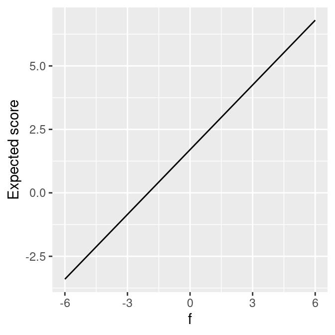
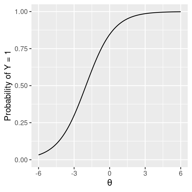
Item Response Function

Also called item characteristic curve

\(Y = 1 + 0.5 f\)

\(\mathrm{logit}(Y) = 1.7 (1 + 0.5 \theta)\)

Benefits of IRT

• Estimates of item parameters (e.g., difficulty) and person parameters (e.g., ability) are independent (at least in theory)
• Useful for linking tests consisted of different items
• Standard error of measurement does not need to be assumed constant across participants
• Useful for examining differential item functioning (i.e., item and test “bias”)

One-Parameter Logistic (1PL) Model

\[\log \frac{P(Y_{ij} = 1)}{P(Y_{ij} = 0)} = Da(\theta_{\color{red}j} - b_{\color{green}i})\]

• \(\theta_{\color{red}j}\): ability/trait level for person \(j\)
• \(b_{\color{green}i}\): difficulty of item \(i\)
  • \(\theta\) level required to have 50% chance of scoring “1” on item \(i\)
• \(a\): discrimination (constant across items in 1PL)
• \(D\): scaling constant (ignored in mirt)¹

Important

Log odds of scoring a 1 = linear function of the distance between (a) person and (b) item.

1. some software set this to 1.7 to make the logistic model comparable to the normal ogive model.

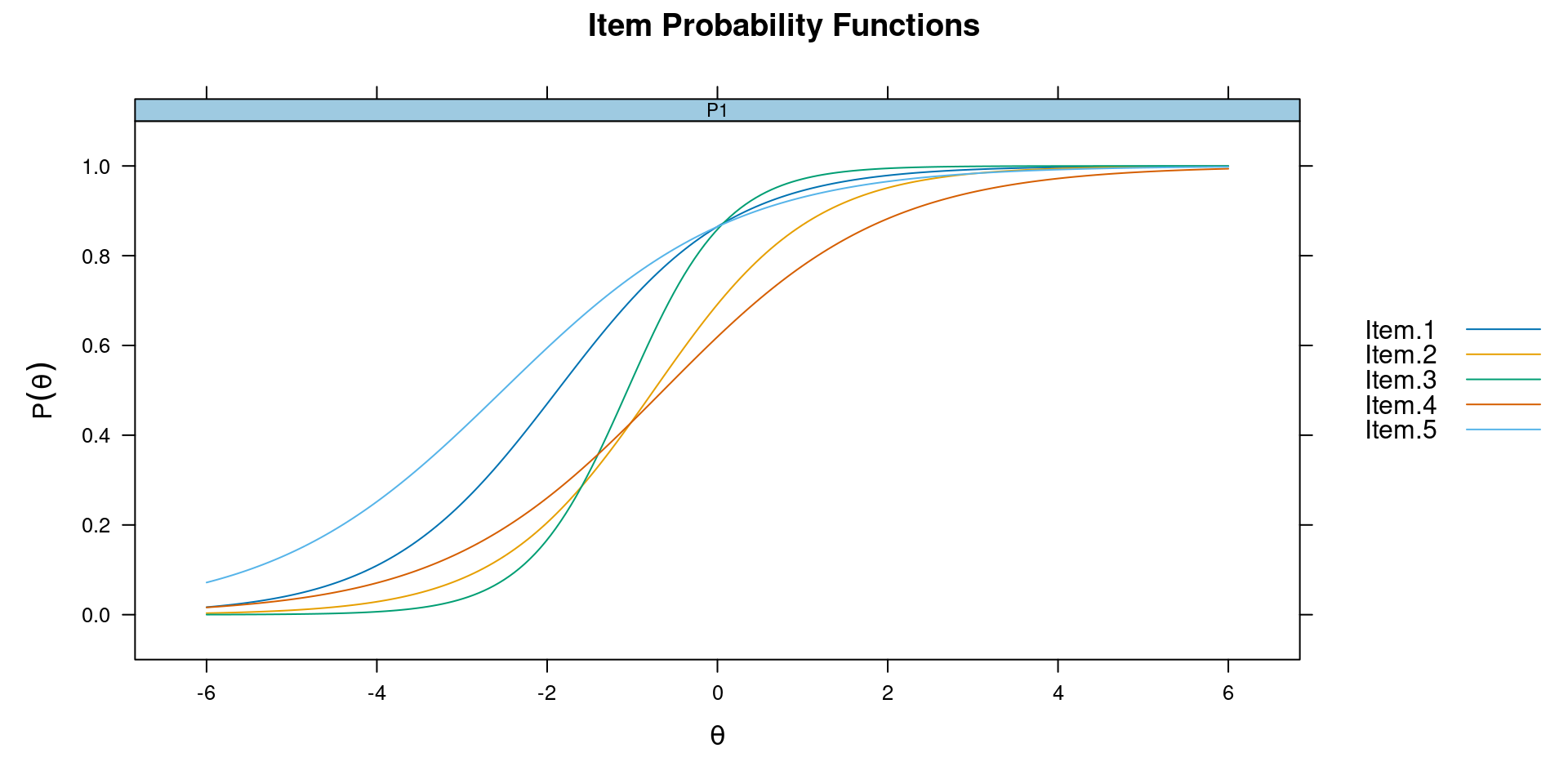
See Figure 14.2 for item response functions

Identification

Similar to CFA, \(\theta\) does not have an intrinsic unit

• One cannot estimate all discrimination parameters and the variance of \(\theta\)
• Relatedly, one cannot estimate all difficulty parameters and the mean of \(\theta\).

Most IRT programs set the mean of \(\theta\) to 0, and variance to 1

Rasch Model

\[\log \frac{P(Y_{ij} = 1)}{P(Y_{ij} = 0)} = \theta_{\color{red}j} - b_{\color{green}i}\]

i.e., with \(Da\) = 1, and variance of \(\theta\) freely estimated.

Note

Despite the mathematical equivalence, Rasch and IRT analyses have somewhat different philosophy. With Rasch, it is believed that Rasch models (e.g., with equal discrimination parameters) are more defensible measurement models, and researchers should strive for constructing items that fit the Rasch models.

On the other hand, with IRT, models are more flexible (and can be made even more so) to accomodate behaviors of test items.

# One-factor
m_rasch <- mirt(dat, model = 1, itemtype = "Rasch")

$items
       a      b g u
Item.1 1 -1.868 0 1
Item.2 1 -0.791 0 1
Item.3 1 -1.461 0 1
Item.4 1 -0.521 0 1
Item.5 1 -1.993 0 1

$means
F1 
 0 

$cov
      F1
F1 1.022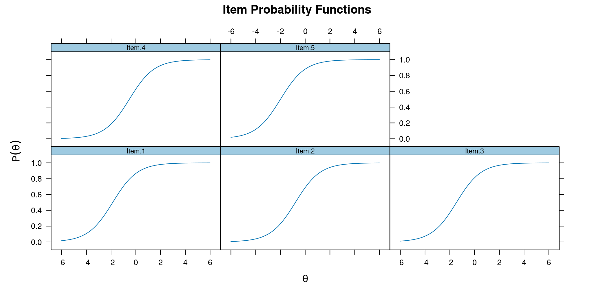

# 1PL
mod_1pl <- "
THETA = 1-5
CONSTRAIN = (1-5, a1)
"
m_1pl <- mirt(dat, mod_1pl)

$items
           a      b g u
Item.1 1.011 -1.848 0 1
Item.2 1.011 -0.782 0 1
Item.3 1.011 -1.445 0 1
Item.4 1.011 -0.516 0 1
Item.5 1.011 -1.971 0 1

$means
THETA 
    0 

$cov
      THETA
THETA     1

plot(m_rasch, type = "trace")

Assumptions

• Correct dimensionality
  • global fit, DIMTEST, parallel analysis, etc
• Local independence
  • Residuals (|Q₃| > .2)
• Correct functional form
  • Item fit (e.g., S-\(\chi^2\))

See R notes

Two-Parameter Logistic Model

\[\log \frac{P(Y_{ij} = 1)}{P(Y_{ij} = 0)} = Da_{\color{red}i}(\theta_{\color{red}j} - b_{\color{green}i})\]

\(a_i\): difference in log odds for 1 unit difference in \(\theta\)

m_2pl <- mirt(dat, model = 1, itemtype = "2PL")

anova(m_rasch, m_2pl)

             AIC    SABIC       HQ      BIC    logLik     X2 df     p
m_rasch 5341.802 5352.192 5352.994 5371.248 -2664.901                
m_2pl   5337.610 5354.927 5356.263 5386.688 -2658.805 12.192  4 0.016

plot(m_2pl, type = "trace", facet_items = FALSE)

Item and Test Information

• Identify items for target trait level
• Assemble short form

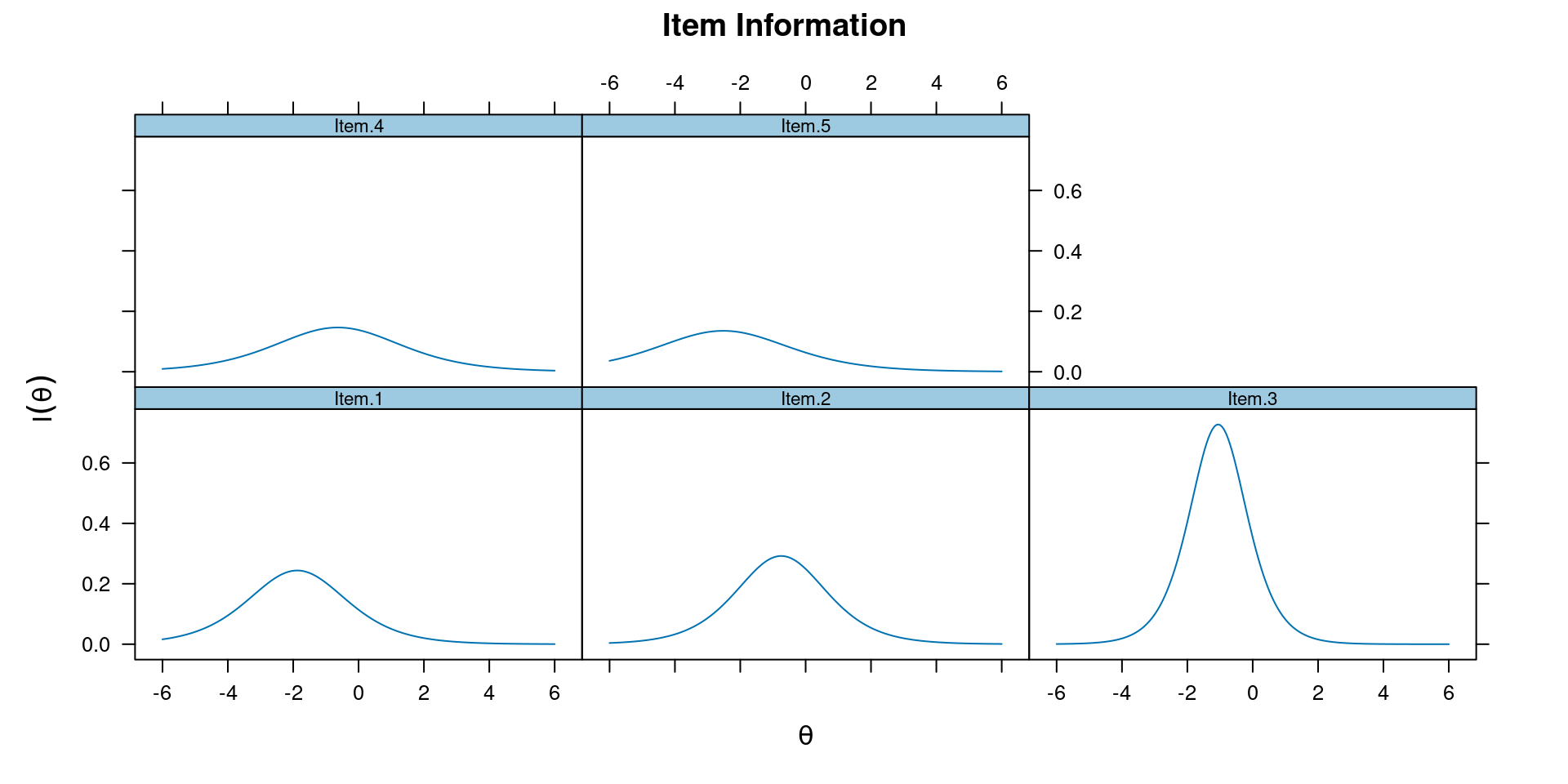
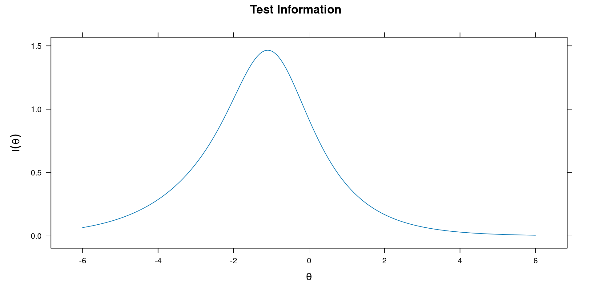
“Reliability”: Var(\(\theta\)) / [Var(\(\theta\)) + 1 / information]

marginal_rxx(m_2pl)

[1] 0.4417618