library(tidyverse)  # for data wrangling and visualization
library(knitr)      # for tables
library(posterior) # for summarizing Bayesian analysesExercise 1
Introduction
In this analysis, we will run a Bayesian analysis to estimate the death rate of patients diagnosed with AIDS in Australia. Let’s start by loading the packages we’ll use for the analysis.
data(Aids2, package = "MASS")We present the results of exploratory data analysis in Section 2 and the regression model in Section 3. See
Exploratory data analysis
The data contains 2843 participants.
Summary statistics
Table 1 displays basic summary statistics.
table(Aids2$state, Aids2$status) |>
kable()| A | D | |
|---|---|---|
| NSW | 664 | 1116 |
| Other | 107 | 142 |
| QLD | 78 | 148 |
| VIC | 233 | 355 |
Modeling
We can fit a simple linear regression model of the form shown in ?@eq-slr.
Table 2 shows the regression output for this model.
prior_a <- 2
prior_b <- 2

posterior_a <- prior_a + sum(Aids2$status == "D")
posterior_b <- prior_b + sum(Aids2$status == "A")

posterior_draws <- rbeta(4000, shape1 = posterior_a, shape2 = posterior_b)

list(theta = posterior_draws) |>
  summarize_draws() |>
kable(digits = 2)| variable | mean | median | sd | mad | q5 | q95 | rhat | ess_bulk | ess_tail |
|---|---|---|---|---|---|---|---|---|---|
| theta | 0.62 | 0.62 | 0.01 | 0.01 | 0.6 | 0.63 | 1 | 4114.48 | 3343.17 |
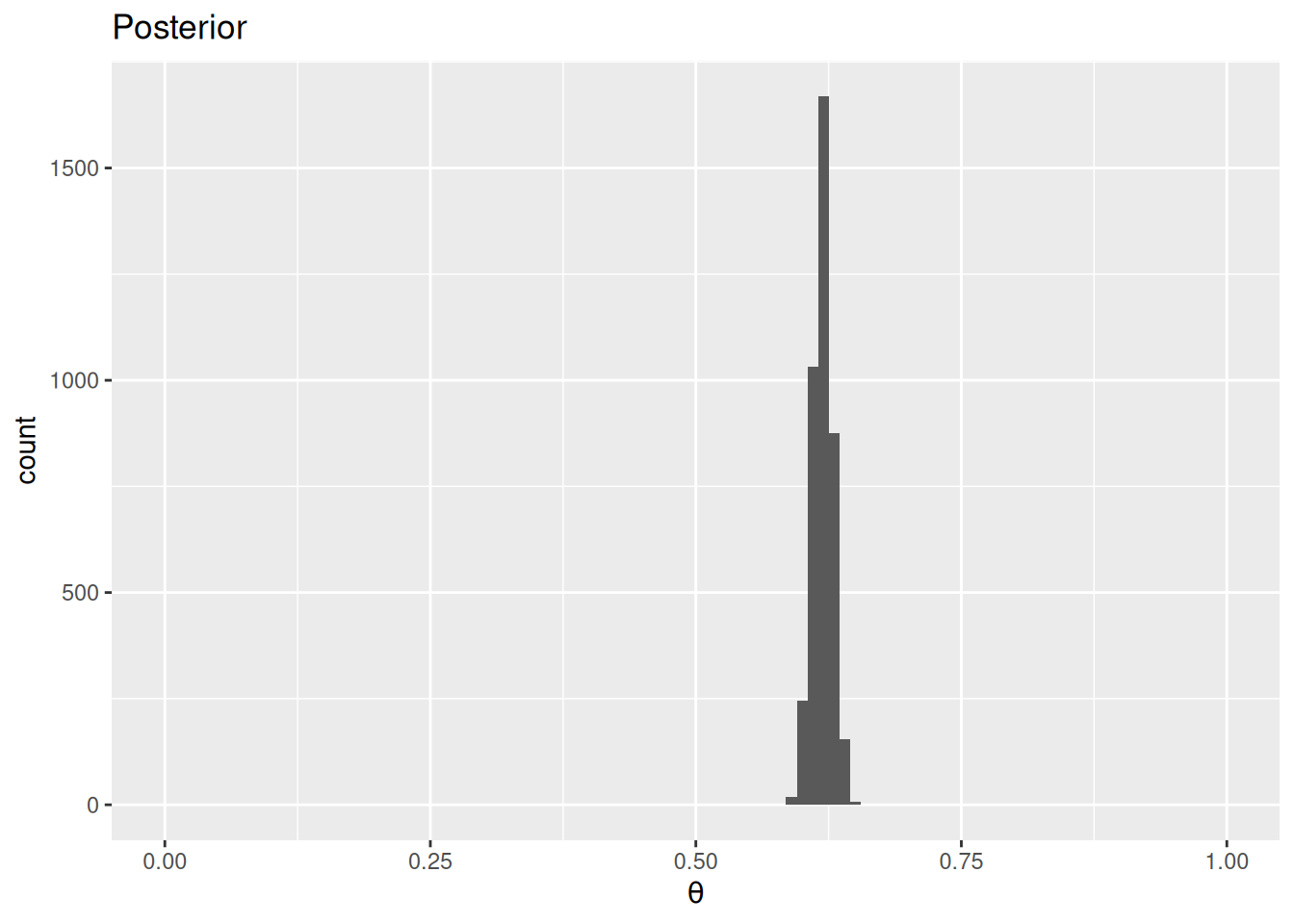
Figure 1 shows the prior and the posterior distributions of the death rate.
prior_draws <- rbeta(4000, shape1 = prior_a, shape2 = prior_b)
ggplot(data.frame(theta = prior_draws), aes(x = theta)) +
  geom_histogram(binwidth = 0.03) +
  labs(title = "Prior", x = expression(theta)) +
  scale_x_continuous(limits = c(0, 1), oob = scales::oob_keep)

ggplot(data.frame(theta = posterior_draws), aes(x = theta)) +
  geom_histogram(binwidth = 0.01) +
  labs(title = "Posterior", x = expression(theta)) +
  scale_x_continuous(limits = c(0, 1), oob = scales::oob_keep)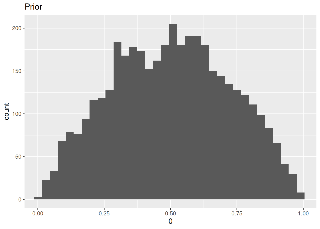
Results
The estimated death rate is 0.62, 95% CI [0.6, 0.64].