Exercise 10

library(here)
library(tidyverse)
library(brms)
options(brms.backend = "cmdstanr", mc.cores = 2)
library(rstan)

Instruction

Answer questions 1-7 below. You can simply submit your responses in text, without using Quarto.

datfile <- here("usc-psyc573-notes/data", "marginalp.xlsx")
marginalp <- readxl::read_excel(datfile)
# Recode `Field` into a factor
marginalp <- marginalp |>
    # Filter out studies without any experiments
    filter(`Number of Experiments` >= 1) |>
    mutate(Field = factor(Field,
        labels = c(
            "Cognitive Psychology",
            "Developmental Psychology",
            "Social Psychology"
        )
    )) |>
    # Rename the outcome
    rename(marginal_p = `Marginals Yes/No`)
marginalp <- marginalp |>
  mutate(Year10 = (Year - 1970) / 10)
marginalp_cog <- filter(marginalp,
                        Field == "Cognitive Psychology")

The following fits the logistic model:

\[ \begin{aligned} \text{marginal\_p}_i & \sim \mathrm{Bern}(\mu_i) \\ \mathrm{logit}(\mu_i) & = \eta_i \\ \eta_i & = \beta_0 + \beta_1 \text{Year10}_{i} \end{aligned} \]

where marginal_p is a binary variable indicating whether a paper contains any marginal \(p\) values (\(.05 < p \leq .10\)), and Year10 = (Year - 1970) / 10. For example, in the Year 2010, Year10 = 4.

m1 <- brm(marginal_p ~ Year10,
    data = marginalp_cog,
    family = bernoulli(link = "logit"),
    prior = c(
        prior(student_t(4, 0, 1), class = "b"),
        prior(student_t(4, 0, 2.5), class = "Intercept")
    ),
    file = "ex10_m1"
)
m1

 Family: bernoulli 
  Links: mu = logit 
Formula: marginal_p ~ Year10 
   Data: marginalp_cog (Number of observations: 87) 
  Draws: 4 chains, each with iter = 2000; warmup = 1000; thin = 1;
         total post-warmup draws = 4000

Regression Coefficients:
          Estimate Est.Error l-95% CI u-95% CI Rhat Bulk_ESS Tail_ESS
Intercept    -1.33      0.44    -2.21    -0.50 1.00     2705     2276
Year10        0.28      0.16    -0.03     0.61 1.00     3038     2826

Draws were sampled using sample(hmc). For each parameter, Bulk_ESS
and Tail_ESS are effective sample size measures, and Rhat is the potential
scale reduction factor on split chains (at convergence, Rhat = 1).

plot(
    conditional_effects(m1, prob = .90),
    points = TRUE,
    point_args = list(height = 0.01, width = 0.05, alpha = 0.05),
    plot = FALSE
)[[1]] +
    scale_x_continuous(
        breaks = 0:4,
        labels = c("1970", "1980", "1990", "2000", "2010")
    ) +
    xlab("Year")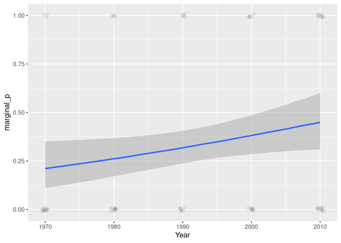

Q1: Why is there no \(\sigma\) parameter?

Q2: Based on the model estimated coefficients, what is the predicted log odds of Y (i.e., having a marginal \(p\) value) for the year 2000?

Q3: What is the predicted probability of Y for the year 2000? [Note: Probability = exp(log odds) / (1 + exp(log odds))]

Q4: What is the predicted probability of Y for the year 2010?

Q5: The probability of Y in 2010 is ____ times the probability of Y in 2000.

Q6: The odds ratio can be computed as \(\exp(\beta_1)\) = _______. Is this number the same as the probability ratio in Q5? Why or why not?

Q7: \(\beta_1 / 4\) = _______. The difference in probability of Y from 2000 to 2010 is _______.