Exercise 2

library(ggplot2)

In this exercise, we will guess the “bias” of a coin he made. “Bias” is defined as the probability of getting a head. We will use grid approximation to perform Bayesian inference updates.

Prior

Q1: Based on the information you have so far, form a prior distribution on the value of \(\theta\) from .05, .15, to .95.

# Possible value of parameter
thetas <- seq(.05, to = .95, by = .10)
# Prior (change the numbers below according to the relative plausibility)
pth <- c(
    `.05` = .1, # for .05
    `.15` = .1, # for .15
    `.25` = .1, # for .25
    `.35` = .1, # for .35
    `.45` = .1, # for .45
    `.55` = .1, # for .55
    `.65` = .1, # for .65
    `.75` = .1, # for .75
    `.85` = .1, # for .85
    `.95` = .1 # for .95
)
# Make sure the probabilities sum to 1; if not, scaled it
sum(pth)

[1] 1

pth <- pth / sum(pth)

The following plots your prior

ggplot(data.frame(th = thetas, prior_prob = pth),
       aes(x = th, y = pth)) +
    geom_col(width = 0.01) +
    labs(x = expression(theta), y = "Prior probability") +
    scale_x_continuous(breaks = thetas) +
    ylim(0, 0.5)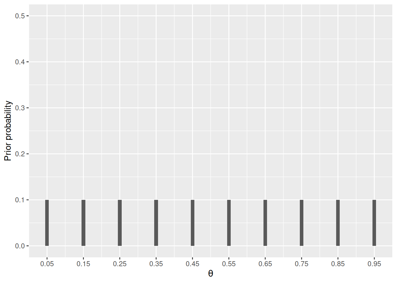

Data

Now, we run the Shiny application with the code below.

shiny::runGitHub("coin_flip", "marklhc")

Q2: In the shiny application, flip the coin twice. Save the data into y1 below (1 = “head”, 0 = “tail”).

(y1 <- c(0, 1))

[1] 0 1

The likelihood function is \[ P(y | \theta) = \theta^z (1 - \theta)^{N - z}, \] where \(N\) is the number of flips, and \(z\) is the number of heads, as implemented in the following function lik:

# Likelihood function
lik <- function(th, y) {
    num_heads <- sum(y)
    num_tails <- length(y) - num_heads
    th ^ num_heads * (1 - th) ^ num_tails
}
pD_given_th <- lik(thetas, y1)  # likelihood values for different thetas

Q3: Explain what th and y represent in the above function.

Figure 1 shows the likelihood function:

ggplot(data.frame(th = thetas, lik = pD_given_th),
       aes(x = th, y = lik)) +
    geom_col(width = 0.01) +
    scale_x_continuous(breaks = thetas) +
    labs(x = expression(theta), y = "Likelihood")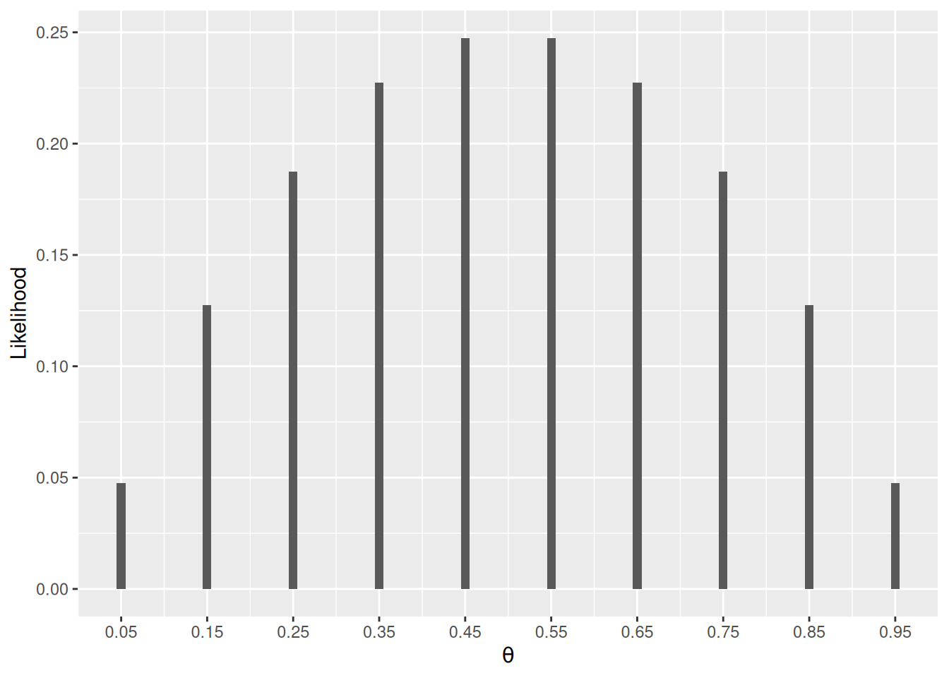

Figure 1

Posterior

Using Bayes’ theorem, we compute the posterior distribution, and make sure the sum of the posterior probabilities is 1.

# Compute the posterior based on Bayes' theorem
pth_given_D <- pD_given_th * pth / sum(pD_given_th * pth)
sum(pth_given_D)

[1] 1

Alternatively, we can compute the products of prior x likelihood, and then scale the values to sum to 1

# Compute the posterior based on Bayes' theorem
pth_given_D2 <- pth * pD_given_th
pth_given_D2 <- pth_given_D2 / sum(pth_given_D2)  # scale to sum to 1

Q4: show that the two approaches give the same posterior probabilities

# [insert code for Q4]

Plot the posterior

ggplot(data.frame(th = thetas, post_prob = pth_given_D),
       aes(x = th, y = post_prob)) +
    geom_col(width = 0.01) +
    scale_x_continuous(breaks = thetas) +
    labs(x = expression(theta), y = "Posterior probability") +
    ylim(0, 0.5)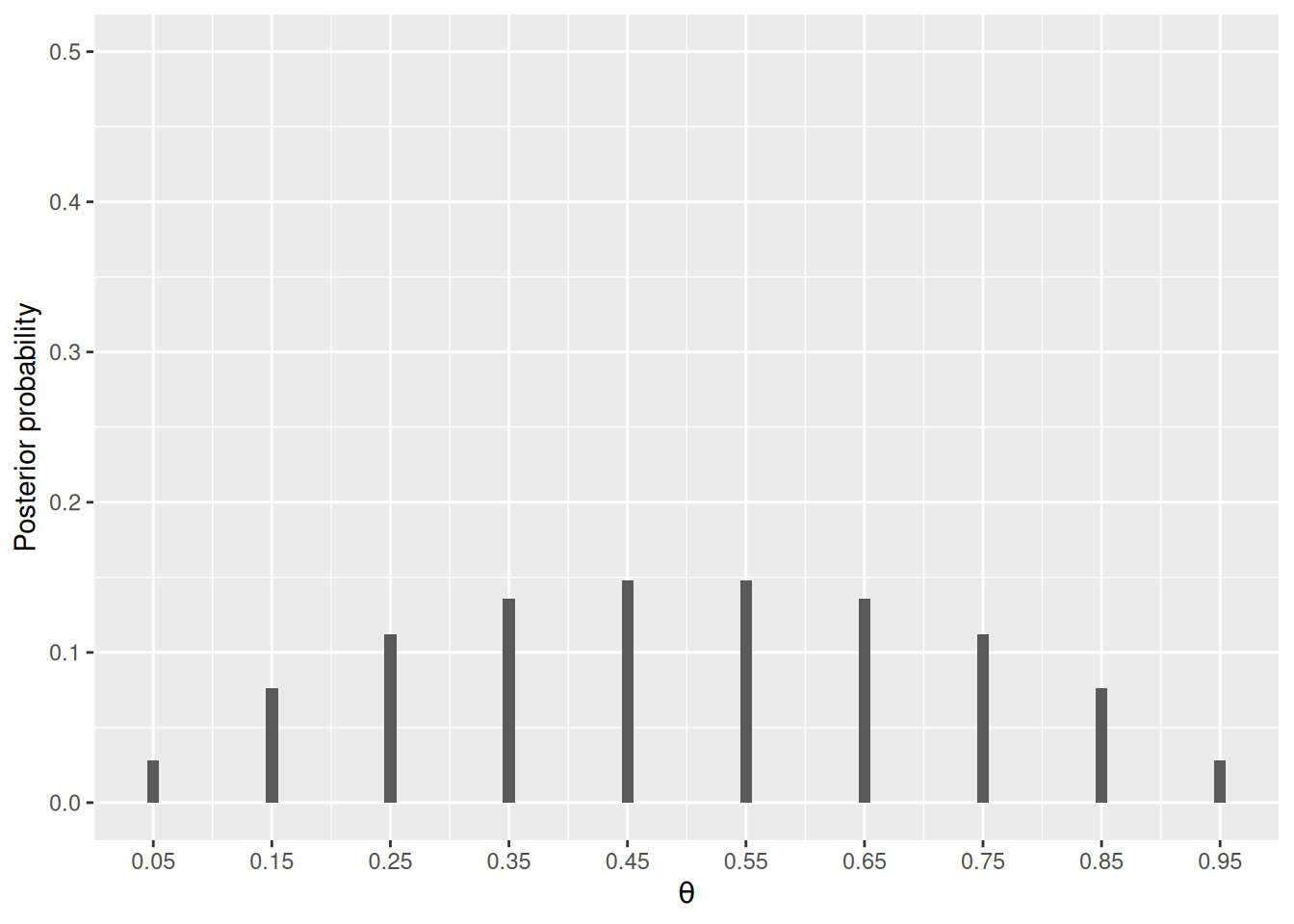

Q5: Use the previous posterior as your new prior. Flip the coin eight more times, and plot the new posterior based on your data.

# Make old posterior the new prior, pth
pth <- pth_given_D
# Record the new data as y2
y2 <- rep(c(0, 1), c(2, 6))
# Obtain the likelihood, pD_given_th
pD_given_th <- lik(thetas, y2)
# Compute the new posterior, pth_given_D

Q6: Use the simulated theta to estimate the mean, median, and standard deviation of the posterior.

sim_thetas <- sample(thetas, size = 10000,
                     prob = pD_given_th * pth, replace = TRUE)
# Obtain the mean, median, and standard deviation

Q7: We consider that the coin is fair if \(\theta\) is between 0.45 and 0.55. The posterior probability that the coin is fair is

# Calculate the probability that the coin is fair