library(here)  # for managing directories
library(tidyverse)
library(readxl)  # for reading excel files
library(brms)
options(brms.backend = "cmdstanr")
library(bayesplot)Exercise 5
In this exercise, please answer questions 1-5 below.. Please make sure you change the YAML option to eval: true. Submit the knitted file (HTML/PDF/WORD) to Blackboard. Be sure to include your name.
A previous paper (https://www.nber.org/papers/w9853.pdf) suggested that instructional ratings were generally higher for those who were viewed as better looking.
Here is the description of some of the variables in the data:
tenured: 1 = tenured professor, 0 = notminority: 1 = yes, 0 = noage: in yearsbtystdave: standardized composite beauty rating based on the ratings of six undergraduatesprofevaluation: evaluation rating of the instructor: 1 (very unsatisfactory) to 5 (excellent)female: 1 = female, 0 = malelower: 1 = lower-division course, 1 = upper-divisionnonenglish: 1 = non-native English speakers, 0 = native-English speakers
You can import the excel data using the readxl::read_excel() function.
beauty <- read_excel(here("data_files", "ProfEvaltnsBeautyPublic.xls"))
# Convert `lower` to factor
beauty$lower <- factor(beauty$lower, levels = c(0, 1),
                       labels = c("upper", "lower"))
Here is a look on profevaluation across upper- and lower-division courses
ggplot(beauty, aes(x = lower, y = profevaluation)) +
    geom_violin() +
    geom_jitter(width = .05, alpha = 0.2)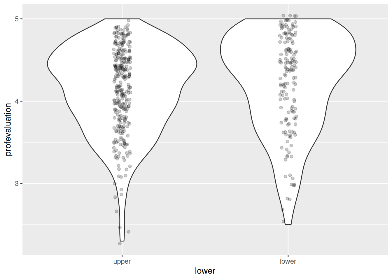
Q1: The following code obtains the priors for a model with lower predicting profevaluation. The model is
\[ \begin{aligned} \text{profevaluation}_i & \sim N(\mu_i, \sigma) \\ \mu_i & = \beta_0 + \beta_1 \text{lower}_i \end{aligned} \]
Describe what each model parameter means, and what prior is used by default in brms.
f1 <- profevaluation ~ lower
get_prior(f1, data = beauty)
Q2: The following simulates some data based on some vague priors, and shows the distributions of the simulated data. Do the priors seem reasonable?
m1_prior <- brm(f1, data = beauty,
                prior = prior(normal(3, 2), class = "Intercept") +
                    prior(normal(0, 1), class = "b",
                          coef = "lowerlower") +
                    prior(student_t(3, 0, 2.5), class = "sigma"),
                sample_prior = "only",
                file = "ex5_m1_prior")
# Prior predictive draws
prior_ytilde <- posterior_predict(m1_prior)Loading required package: rstanLoading required package: StanHeaders
rstan version 2.32.5 (Stan version 2.32.2)For execution on a local, multicore CPU with excess RAM we recommend calling
options(mc.cores = parallel::detectCores()).
To avoid recompilation of unchanged Stan programs, we recommend calling
rstan_options(auto_write = TRUE)
For within-chain threading using `reduce_sum()` or `map_rect()` Stan functions,
change `threads_per_chain` option:
rstan_options(threads_per_chain = 1)
Attaching package: 'rstan'The following object is masked from 'package:tidyr':
extract# lower = lower
prior_ytilde_lower <- prior_ytilde[, beauty$lower == "lower"]
ppd_dens_overlay(prior_ytilde_lower)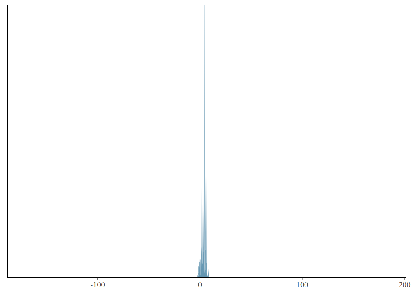
# lower = upper
prior_ytilde_upper <- prior_ytilde[, beauty$lower == "upper"]
ppd_dens_overlay(prior_ytilde_upper)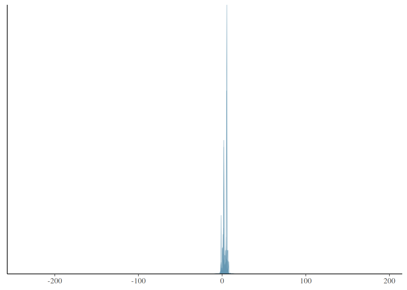
Q3: Modify the code below to assign more reasonable priors, and run the code to draw posterior samples.
m1 <- brm(f1, data = beauty,
prior = prior(normal(3, 2), class = "Intercept") +
prior(normal(0, 1), class = "b", coef = "lowerlower") +
prior(student_t(3, 0, 2.5), class = "sigma"),
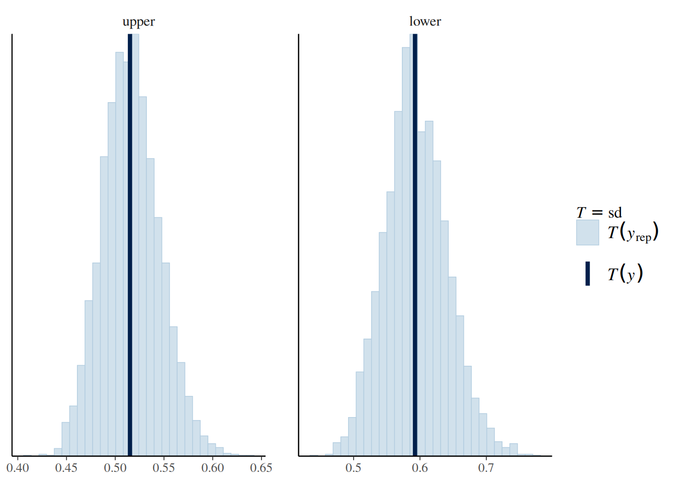
file = "ex5_m1")Q4: Below are plots showing the predictive distribution of the sample SD by lower and upper divisions. Does it appear that the error variance is different for upper-division and lower-division courses?
# sample SD from the posterior predictive distribution
pp_check(m1, type = "stat_grouped", group = "lower", stat = "sd")
Using all posterior draws for ppc type 'stat_grouped' by default.`stat_bin()` using `bins = 30`. Pick better value with `binwidth`.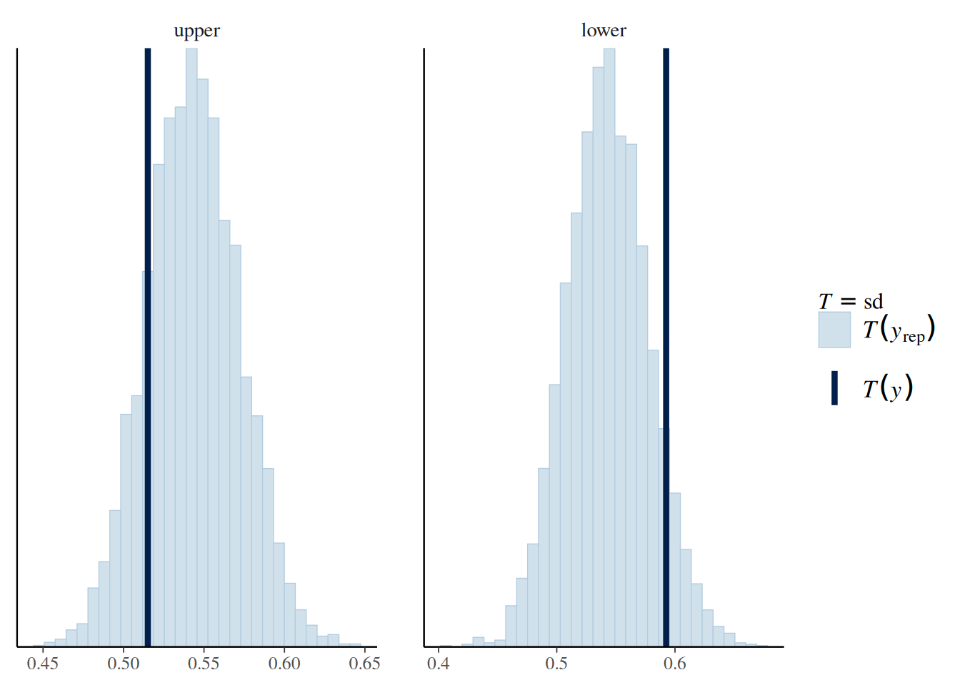
Q5: The following model includes lower as a predictor for sigma. Does it appear that the error variance/sd is related to lower?
\[ \begin{aligned} \text{profevaluation}_i & \sim N(\mu_i, \sigma_i) \\ \mu_i & = \beta_0 + \beta_1 \text{lower}_i \\ \log \sigma_i & = \beta_0^s + \beta_1^s \text{lower}_i \end{aligned} \]
m2 <- brm(bf(f1, sigma ~ lower), data = beauty,
          file = "ex5_m2")
# Compare models 1 and 2
loo(m1, m2)Output of model 'm1':
Computed from 4000 by 463 log-likelihood matrix.
Estimate SE
elpd_loo -375.9 15.7
p_loo 3.1 0.3
looic 751.8 31.4
------
MCSE of elpd_loo is 0.0.
MCSE and ESS estimates assume MCMC draws (r_eff in [0.8, 1.2]).
All Pareto k estimates are good (k < 0.7).
See help('pareto-k-diagnostic') for details.
Output of model 'm2':
Computed from 4000 by 463 log-likelihood matrix.
Estimate SE
elpd_loo -374.8 15.9
p_loo 4.0 0.5
looic 749.6 31.8
------
MCSE of elpd_loo is 0.0.
MCSE and ESS estimates assume MCMC draws (r_eff in [0.9, 1.4]).
All Pareto k estimates are good (k < 0.7).
See help('pareto-k-diagnostic') for details.
Model comparisons:
elpd_diff se_diff
m2 0.0 0.0
m1 -1.1 2.1 print(m2) Family: gaussian
Links: mu = identity; sigma = log
Formula: profevaluation ~ lower
sigma ~ lower
Data: beauty (Number of observations: 463)
Draws: 4 chains, each with iter = 2000; warmup = 1000; thin = 1;
total post-warmup draws = 4000
Regression Coefficients:
Estimate Est.Error l-95% CI u-95% CI Rhat Bulk_ESS Tail_ESS
Intercept 4.14 0.03 4.09 4.20 1.00 5383 3198
sigma_Intercept -0.66 0.04 -0.74 -0.58 1.00 4555 3103
lowerlower 0.10 0.06 -0.02 0.21 1.00 4267 3213
sigma_lowerlower 0.14 0.07 0.00 0.28 1.00 4498 2701
Draws were sampled using sample(hmc). For each parameter, Bulk_ESS
and Tail_ESS are effective sample size measures, and Rhat is the potential
scale reduction factor on split chains (at convergence, Rhat = 1).pp_check(m2, type = "stat_grouped", group = "lower", stat = "sd")Using all posterior draws for ppc type 'stat_grouped' by default.`stat_bin()` using `bins = 30`. Pick better value with `binwidth`.