| Estimate | Est.Error | Q2.5 | Q97.5 | |
|---|---|---|---|---|
| Intercept | 2.79 | 0.46 | 1.91 | 3.73 |
| Southsouth | 3.15 | 1.50 | 0.18 | 6.12 |
| MedianAgeMarriage | -0.71 | 0.17 | -1.07 | -0.37 |
| Southsouth:MedianAgeMarriage | -1.20 | 0.58 | -2.36 | -0.03 |
Exercise 6
The analyses in this exercise are from the example in the note “9 Multiple Predictors” (https://marklhc.quarto.pub/psyc573-2024fall/docs/06b-multiple-predictors.html#conditional-effectssimple-slopes)
S = 0 for non-southern states; S = 1 for southern states
Consider the interaction model
\[ \begin{aligned} D_i & \sim N(\mu_i, \sigma) \\ \mu_i & = \beta_0 + \beta_1 S_i + \beta_2 A_i + \beta_3 S_i \times A_i \end{aligned} \]
Q1
Express, in terms of the model parameters (e.g., \(\beta_0\), \(\beta_1\)),
the predicted divorce rate (\(\mu\)) for a southern state with
MedianAgeMarriage= 2.5: _____________________the predicted \(\mu\) for a non-southern state with
MedianAgeMarriage= 2.5: _____________________the difference between (a) and (b): ____________________________
Q2
The following shows the estimated coefficients (from brms)
and the interaction plot:
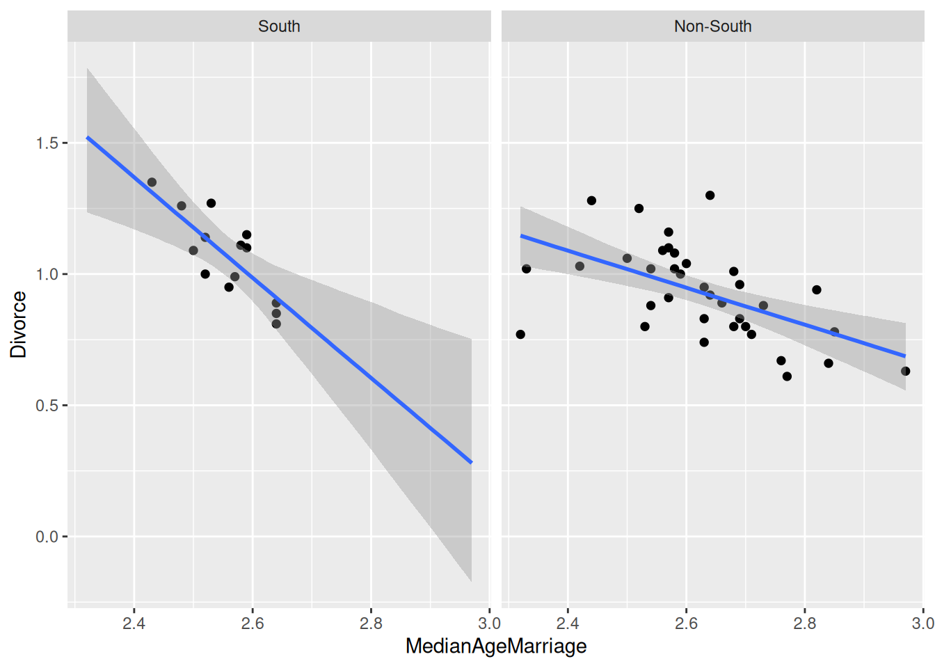
Label \(\beta_0\), \(\beta_1\), \(\beta_2\), \(\beta_3\), and \(\sigma\) in the graph above (or describe where they are in your words).