| Person | Math Attitude | Y (if T = 1) | Y (if T = 0) | Y(1) - Y(0) |
|---|---|---|---|---|
| 1 | 4 | 75 | 70 | 5 |
| 2 | 7 | 80 | 88 | -8 |
| 3 | 3 | 70 | 75 | -5 |
| 4 | 9 | 90 | 92 | -2 |
| 5 | 5 | 85 | 82 | 3 |
| 6 | 6 | 82 | 85 | -3 |
| 7 | 8 | 95 | 90 | 5 |
| 8 | 2 | 78 | 78 | 0 |
| Average | 5.5 | 81.875 | 82.5 | -0.625 |
Causal Inference
PSYC 573
Directed Acyclic Graph
Allows researchers to encode causal assumptions of the data
- Based on knowledge of the data and the variables
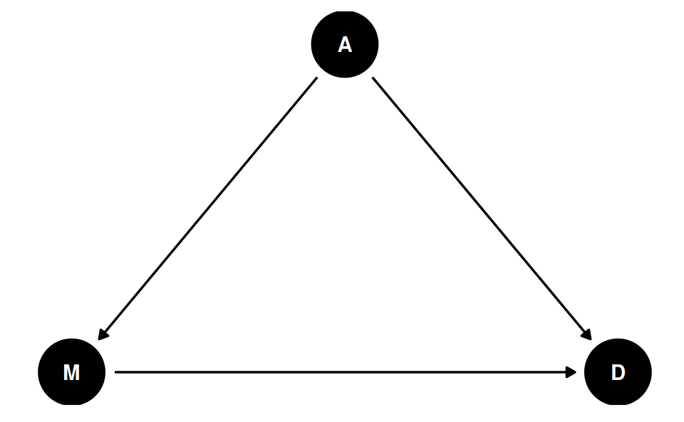
Data from the 2009 American Community Survey (ACS)
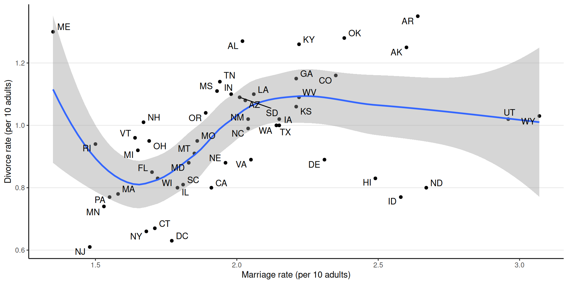
Does marriage cause divorce?
- A = Median age of marriage
- M = Marriage rate
- D = Divorce rate
“Weak” assumptions
- A may directly influence M
- A may directly influence D
- M may directly influence D
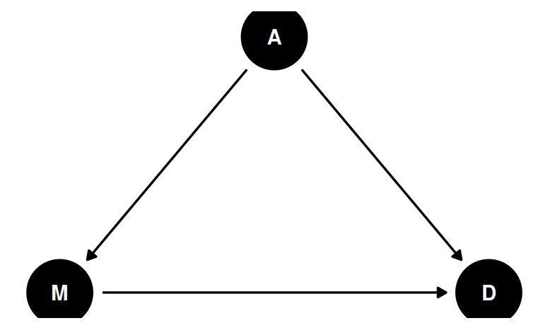
“Strong” assumptions
Absence of a link
- E.g., M does not directly influence A
- E.g., A is the only relevant variable in the causal pathway M → D
Framing Experiment
- X: exposure to a negatively framed news story about immigrants
- Y: anti-immigration political action
No Randomization
Randomization
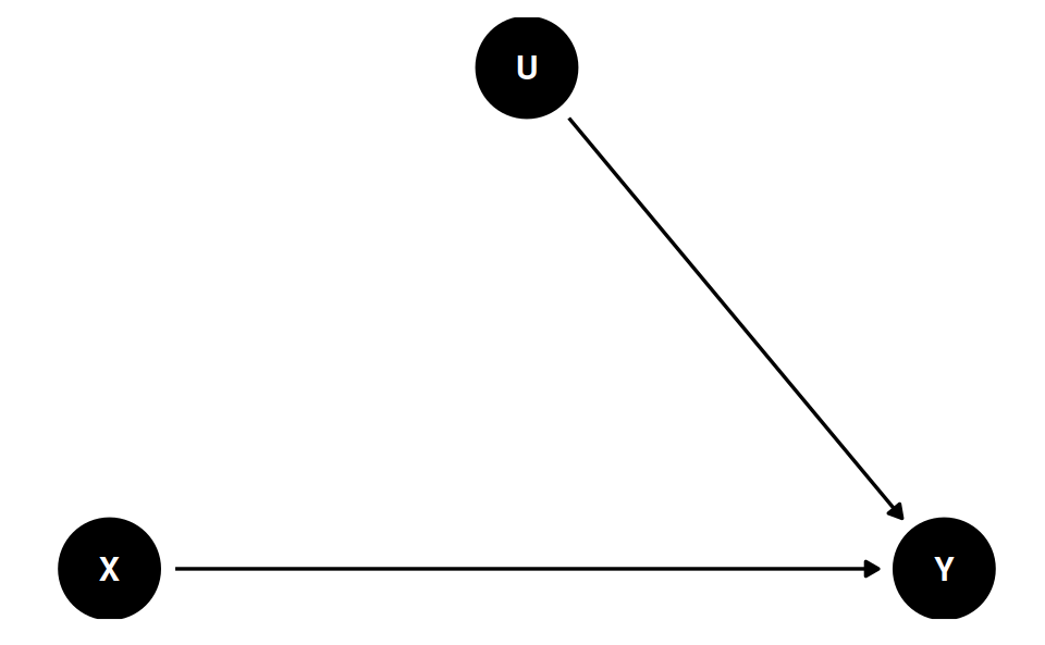
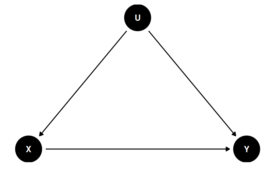
Back-Door Criterion
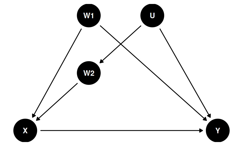
The causal effect of X → Y can be obtained by blocking all the backdoor paths that do not involve descendants of X
- Randomization: (when done successfully) eliminates all paths entering X
- Conditioning (holding constant)
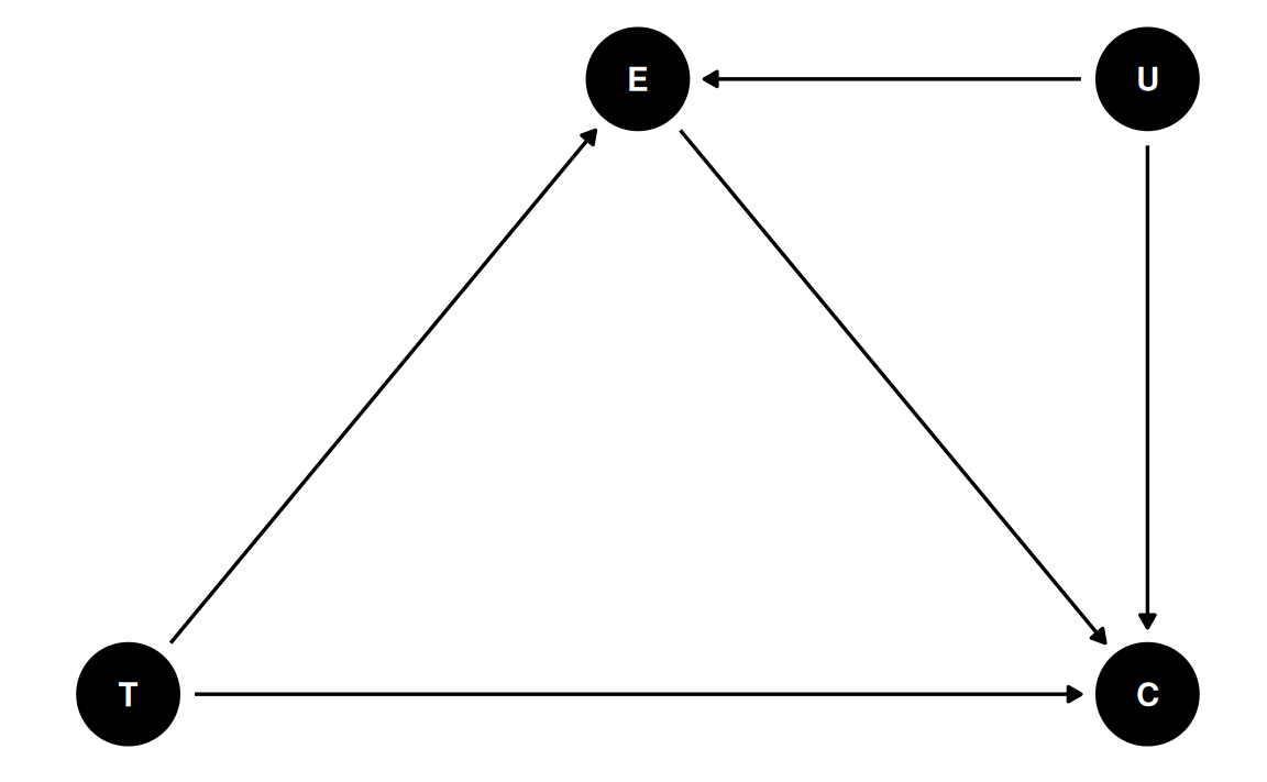
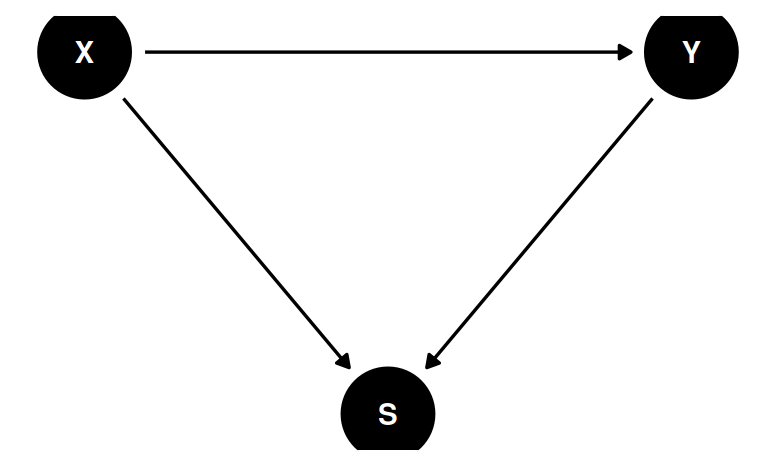
Mediation
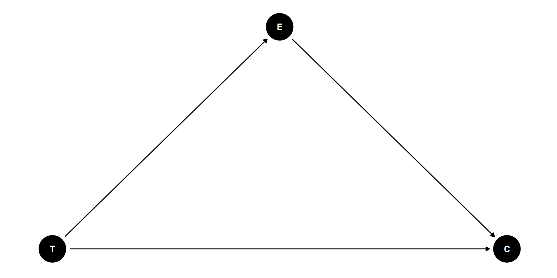
In the DAG, E is a post-treatment variable potentially influenced by T
- E is a potential mediator
Important
A mediator is very different from a confounder
Sensitivity Analysis
Assign priors representing plausible magnitude of confounding (see notes for an example)
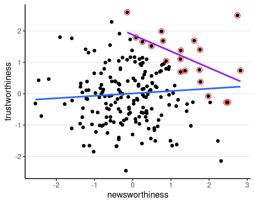
Collider Bias
E.g., Is the most newsworthy research the least trustworthy?
Instrumental Variables
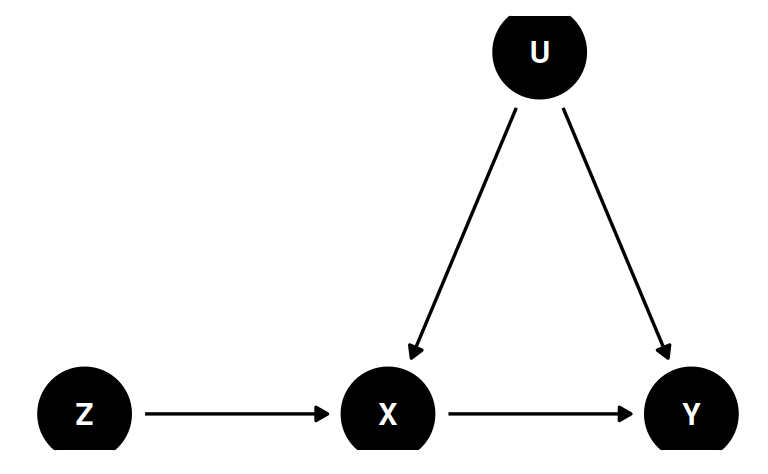
- X = Career Adaptability
- Y = Job Satisfaction
- Z (instrument) = Conscientiousness
- U = Confounding
Instrument
- Plausible cause of X
- Can only affect Y through X