Generalized Linear Model (GLM)

PSYC 573

GLM

Three components:

• Conditional distribution of \(Y\)
• Link function
• Linear predictor (\(\eta\))

Some Examples

Outcome type	Support	Distributions	Link
continuous	[\(-\infty\), \(\infty\)]	Normal	Identity
count (fixed duration)	{0, 1, \(\ldots\)}	Poisson	Log
count (known # of trials)	{0, 1, \(\ldots\), \(N\)}	Binomial	Logit
binary	{0, 1}	Bernoulli	Logit
ordinal	{0, 1, \(\ldots\), \(K\)}	categorical	Logit
nominal	\(K\)-vector of {0, 1}	categorical	Logit
multinomial	\(K\)-vector of {0, 1, \(\ldots\), \(K\)}	categorical	Logit

Mathematical Form (One Predictor)

\[ \begin{aligned} Y_i & \sim \mathrm{Dist}(\mu_i, \tau) \\ g(\mu_i) & = \eta_i \\ \eta_i & = \beta_0 + \beta_1 X_{i} \end{aligned} \]

• \(\mathrm{Dist}\): conditional distribution of \(Y \mid X\) (e.g., normal, Bernoulli, \(\ldots\))
  • I.e., distribution of prediction error; not the marginal distribution of \(Y\)
• \(\mu_i\): mean parameter for the \(i\)th observation
• \(\eta_i\): linear predictor
• \(g(\cdot)\): link function
• (\(\tau\): dispersion parameter)

Illustration

Next few slides contain example GLMs, with the same predictor \(X\)

num_obs <- 100
x <- runif(num_obs, min = 1, max = 5)  # uniform x
beta0 <- 0.2; beta1 <- 0.5

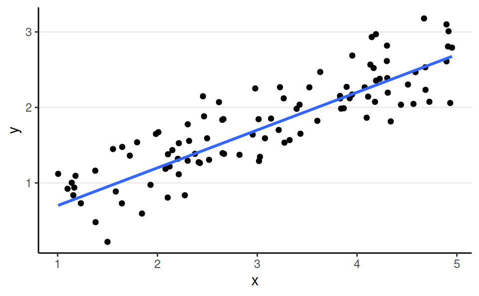
Normal, Identity Link

aka linear regression

\[ \begin{aligned} Y_i & \sim N(\mu_i, \sigma) \\ \mu_i & = \eta_i \\ \eta_i & = \beta_0 + \beta_1 X_{i} \end{aligned} \]

eta <- beta0 + beta1 * x
mu <- eta
y <- rnorm(num_obs, mean = mu, sd = 0.3)

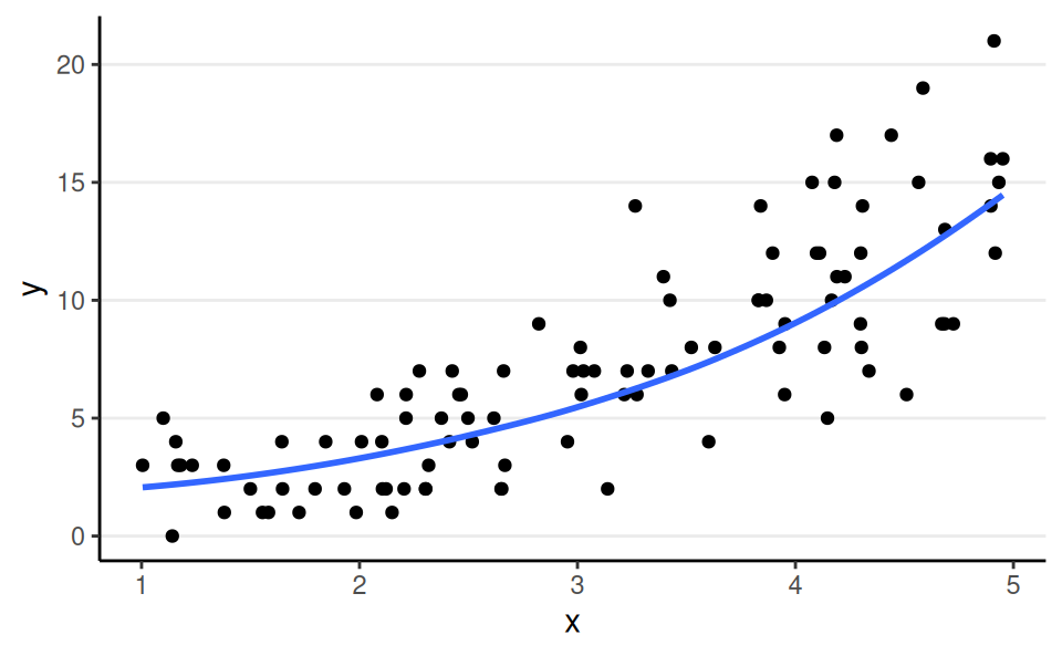
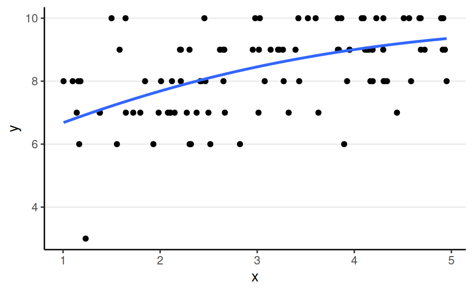
Poisson, Log Link

aka poisson regression

\[ \begin{aligned} Y_i & \sim \mathrm{Pois}(\mu_i) \\ \log(\mu_i) & = \eta_i \\ \eta_i & = \beta_0 + \beta_1 X_{i} \end{aligned} \]

eta <- beta0 + beta1 * x
mu <- exp(eta)  # inverse link
y <- rpois(num_obs, lambda = mu)

Bernoulli, Logit Link

aka binary logistic regression

\[ \begin{aligned} Y_i & \sim \mathrm{Bern}(\mu_i) \\ \log\left(\frac{\mu_i}{1 - \mu_i}\right) & = \eta_i \\ \eta_i & = \beta_0 + \beta_1 X_{i} \end{aligned} \]

eta <- beta0 + beta1 * x
mu <- plogis(eta)  # inverse link is logistic
y <- rbinom(num_obs, size = 1, prob = mu)

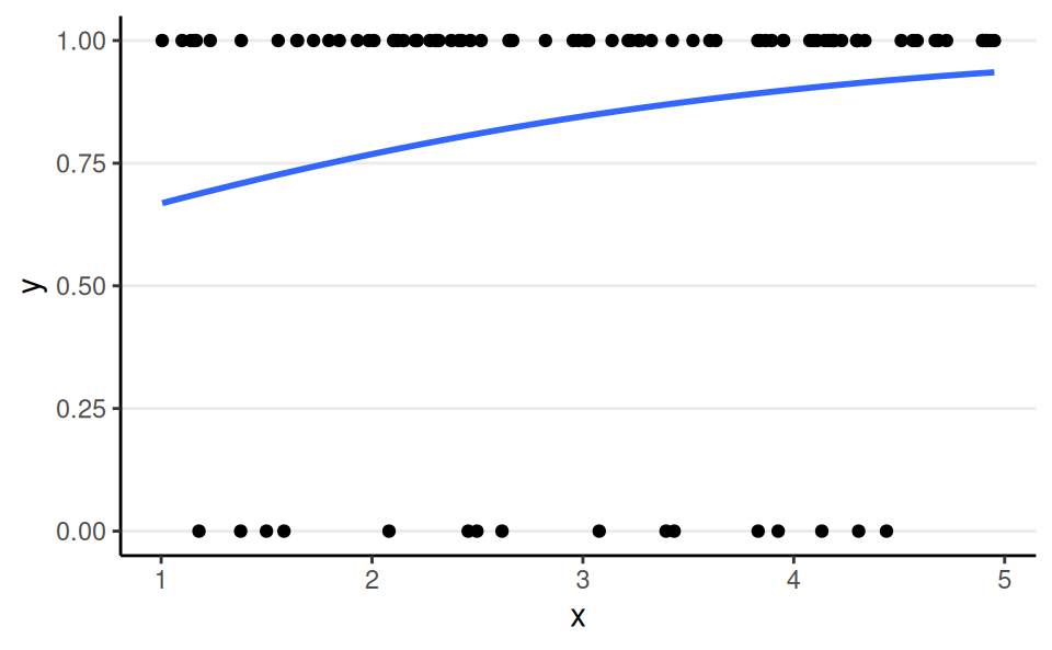
Binomial, Logit Link

aka binomial logistic regression

\[ \begin{aligned} Y_i & \sim \mathrm{Bin}(N, \mu_i) \\ \log\left(\frac{\mu_i}{1 - \mu_i}\right) & = \eta_i \\ \eta_i & = \beta_0 + \beta_1 X_{i} \end{aligned} \]

num_trials <- 10
eta <- beta0 + beta1 * x
mu <- plogis(eta)  # inverse link is logistic
y <- rbinom(num_obs, size = num_trials, prob = mu)

Remarks

Different link functions can be used

• E.g., identity link or probit link for Bernoulli variables

Linearity is a strong assumption

• GLM can allow \(\eta\) and \(X\) to be nonlinearly related, as long as it’s linear in the coefficients
  • E.g., \(\eta_i = \beta_0 + \beta_1 \log(X_{i})\)
  • E.g., \(\eta_i = \beta_0 + \beta_1 X_i + \beta_2 X_i^2\)
  • But not something like \(\eta_i = \beta_0 \log(\beta_1 + x_i)\)

Logistic Regression

See exercise

Poisson Regression

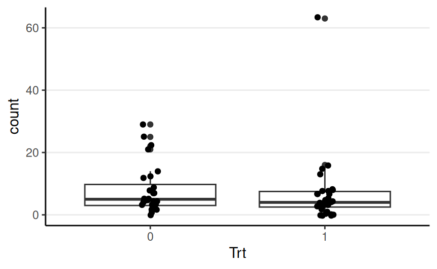
• count: The seizure count between two visits
• Trt: Either 0 or 1 indicating if the patient received anticonvulsant therapy

\[ \begin{aligned} \text{count}_i & \sim \mathrm{Pois}(\mu_i) \\ \log(\mu_i) & = \eta_i \\ \eta_i & = \beta_0 + \beta_1 \text{Trt}_{i} \end{aligned} \]

Poisson with log link

Predicted seizure rate = \(\exp(\beta_0 + \beta_1) = \exp(\beta_0) \exp(\beta_1)\) for Trt = 1; \(\exp(\beta_0)\) for Trt = 0

\(\beta_1\) = mean difference in log rate of seizure; \(\exp(\beta_1)\) = ratio in rate of seizure

m2 <- brm(count ~ Trt, data = epilepsy4,
          family = poisson(link = "log"))

 Family: poisson 
  Links: mu = log 
Formula: count ~ Trt 
   Data: epilepsy4 (Number of observations: 59) 
  Draws: 4 chains, each with iter = 2000; warmup = 1000; thin = 1;
         total post-warmup draws = 4000

Regression Coefficients:
          Estimate Est.Error l-95% CI u-95% CI Rhat Bulk_ESS Tail_ESS
Intercept     2.07      0.07     1.94     2.21 1.00     4022     2321
Trt1         -0.17      0.10    -0.36     0.02 1.00     3435     2620

Draws were sampled using sample(hmc). For each parameter, Bulk_ESS
and Tail_ESS are effective sample size measures, and Rhat is the potential
scale reduction factor on split chains (at convergence, Rhat = 1).

Poisson with identity link

In this case, with one binary predictor, the link does not matter to the fit

\[ \begin{aligned} \text{count}_i & \sim \mathrm{Pois}(\mu_i) \\ \mu_i & = \eta_i \\ \eta_i & = \beta_0 + \beta_1 \text{Trt}_{i} \end{aligned} \]

\(\beta_1\) = mean difference in the rate of seizure in two weeks

m3 <- brm(count ~ Trt, data = epilepsy4,
          family = poisson(link = "identity"))

	log link	identity link
b_Intercept	2.07	7.95
	[1.94, 2.21]	[6.99, 9.08]
b_Trt1	−0.17	−1.24
	[−0.36, 0.02]	[−2.59, 0.07]
Num.Obs.	59	59
R2	0.004	0.004
ELPD	−345.8	−343.8
ELPD s.e.	96.0	94.2
LOOIC	691.5	687.7
LOOIC s.e.	192.0	188.3
WAIC	690.2	689.5
RMSE	9.54	9.56