Hierarchical Models

PSYC 573

2024-09-17

Therapeutic Touch Example (N = 28)

Data Points From One Person

\(y\): whether the guess of which hand was hovered over was correct

Person S01

y	s
1	S01
0	S01
0	S01
0	S01
0	S01
0	S01
0	S01
0	S01
0	S01
0	S01

Binomial Model

We can use a Bernoulli model: \[ y_i \sim \mathrm{Bern}(\theta) \] for \(i = 1, \ldots, N\)

Assuming exchangeability given \(\theta\), more succint to write \[ z \sim \mathrm{Bin}(N, \theta) \] for \(z = \sum_{i = 1}^N y_i\)

• Bernoulli: Individual trial
• Binomial: total count of “1”s

Prior: Beta(1, 1)

1 success, 9 failures

Posterior: Beta(2, 10)

Multiple People

We could repeat the binomial model for each of the 28 participants, to obtain posteriors for \(\theta_1\), \(\ldots\), \(\theta_{28}\)

But . . .

We’ll continue the therapeutic touch example. To recap, we have 28 participants, each of them go through 10 trials to guess which of their hands was hovered above. The histogram shows the distribution of the proportion correct.

Do we think our belief about \(\theta_1\) would inform our belief about \(\theta_2\), etc?

After all, human beings share 99.9% of genetic makeup

Three Positions of Pooling

• No pooling: each individual is completely different; inference of \(\theta_1\) should be independent of \(\theta_2\), etc

• Complete pooling: each individual is exactly the same; just one \(\theta\) instead of 28 \(\theta_j\)’s

• Partial pooling: each individual has something in common but also is somewhat different

No Pooling

Complete Pooling

Partial Pooling

Partial Pooling in Hierarchical Models

Hierarchical Priors: \(\theta_j \sim \mathrm{Beta2}(\mu, \kappa)\)

Beta2: reparameterized Beta distribution

• mean \(\mu = a / (a + b)\)
• concentration \(\kappa = a + b\)

Expresses the prior belief:

Individual \(\theta\)s follow a common Beta distribution with mean \(\mu\) and concentration \(\kappa\)

How to Choose \(\kappa\)

If \(\kappa \to \infty\): everyone is the same; no individual differences (i.e., complete pooling)

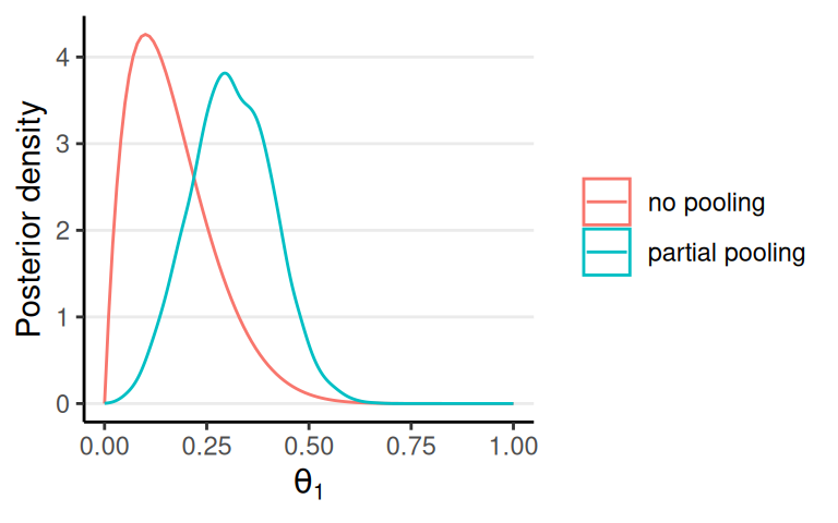
If \(\kappa = 0\): everybody is different; nothing is shared (i.e., no pooling)

We can fix a \(\kappa\) value based on our belief of how individuals are similar or different

A more Bayesian approach is to treat \(\kappa\) as an unknown, and use Bayesian inference to update our belief about \(\kappa\)

Generic prior by Kruschke (2015): \(\kappa\) \(\sim\) Gamma(0.01, 0.01)

Sometimes you may want a stronger prior like Gamma(1, 1), if it is unrealistic to do no pooling

Full Model

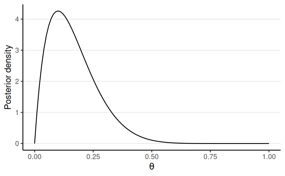
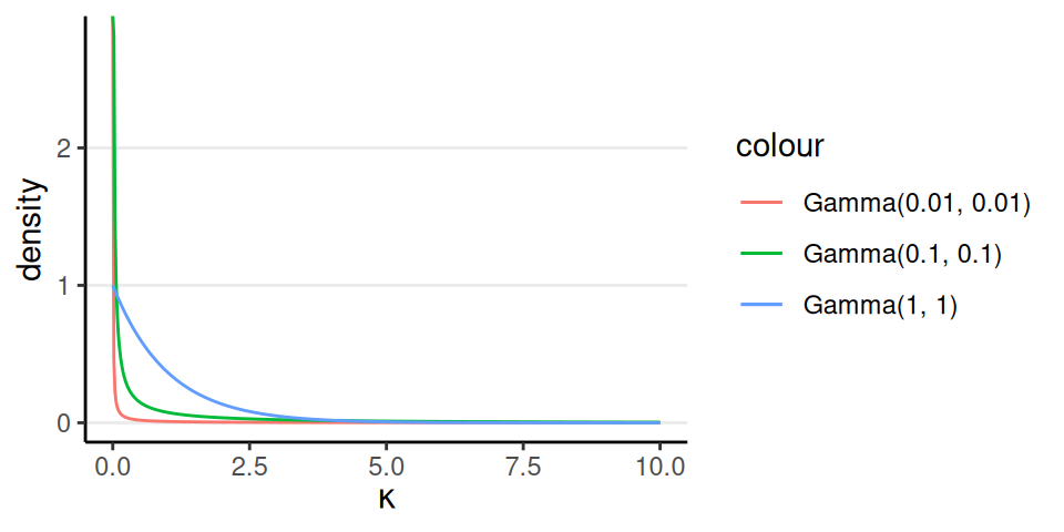
Model: \[ \begin{aligned} z_j & \sim \mathrm{Bin}(N_j, \theta_j) \\ \theta_j & \sim \mathrm{Beta2}(\mu, \kappa) \end{aligned} \] Prior: \[ \begin{aligned} \mu & \sim \mathrm{Beta}(1.5, 1.5) \\ \kappa & \sim \mathrm{Gamma}(0.01, 0.01) \end{aligned} \]

Here’s our model. For each person j, the number of correct responses follows a binoial distribution in N equals 10 trials. The probability, or the ability to sense the experimenter’s hand, is captured by theta j.

Now, we assume the theta js come from a common Beta distribution. Beta here is parameterized with the common mean mu, and the concentration kappa that controls how much to pool.

As for the priors, because mu is the common mean of the thetas, it is again between 0 and 1. I set a weak Beta(1.5, 1.5) prior, which corresponds to half a success and half a failure. If you have stronger belief that the data mostly reflect random guessing, you can put something like Beta(5, 5).

The gamma prior for kappa is recommended by your text as a weak default prior.

data {
  int<lower=0> J;  // number of clusters (e.g., studies, persons)
  array[J] int y;  // number of "1"s in each cluster
  array[J] int N;  // sample size for each cluster
}
parameters {
  // cluster-specific probabilities
  vector<lower=0, upper=1>[J] theta;
  real<lower=0, upper=1> mu;  // overall mean probability
  real<lower=0> kappa;        // overall concentration
}
model {
  y ~ binomial(N, theta);  // each observation is binomial
  // Priors
  theta ~ beta_proportion(mu, kappa);
  mu ~ beta(1.5, 1.5);      // weak prior
  kappa ~ gamma(.1, .1);  // prior recommended by Kruschke
}
generated quantities {
  // Prior and posterior predictive
  real<lower=0, upper=1> prior_mu = beta_rng(1.5, 1.5);
  real<lower=0> prior_kappa = gamma_rng(.1, .1);
  vector<lower=0, upper=1>[J] prior_theta;
  for (j in 1:J) {
    prior_theta[j] = beta_proportion_rng(prior_mu, prior_kappa);
  }
  array[J] int prior_ytilde = binomial_rng(N, prior_theta);
  // Posterior predictive
  array[J] int ytilde = binomial_rng(N, theta);
}

Here is the Stan code. The inputs are J, the number of people, y, which is actually z in our model for the individual counts, but I use y just because y is usually the outcome in Stan. N is the number of trials per person, and here N[J] means the number of trials can be different across individuals.

The parameters and the model block pretty much follow the mathematical model. The beta_proportion() function is what I said Beta2 as the beta distribution with the mean and the concentration as the parameters.

You may want to pause here to make sure you understand the Stan code.

hbin_mod <- cmdstan_model("stan_code/hierarchical-binomial.stan")

tt_fit <- hbin_mod$sample(
    data = list(J = nrow(tt_agg),
                y = tt_agg$y,
                N = tt_agg$n,
                prior_only = FALSE),
    seed = 1716,  # for reproducibility
    refresh = 1000
)

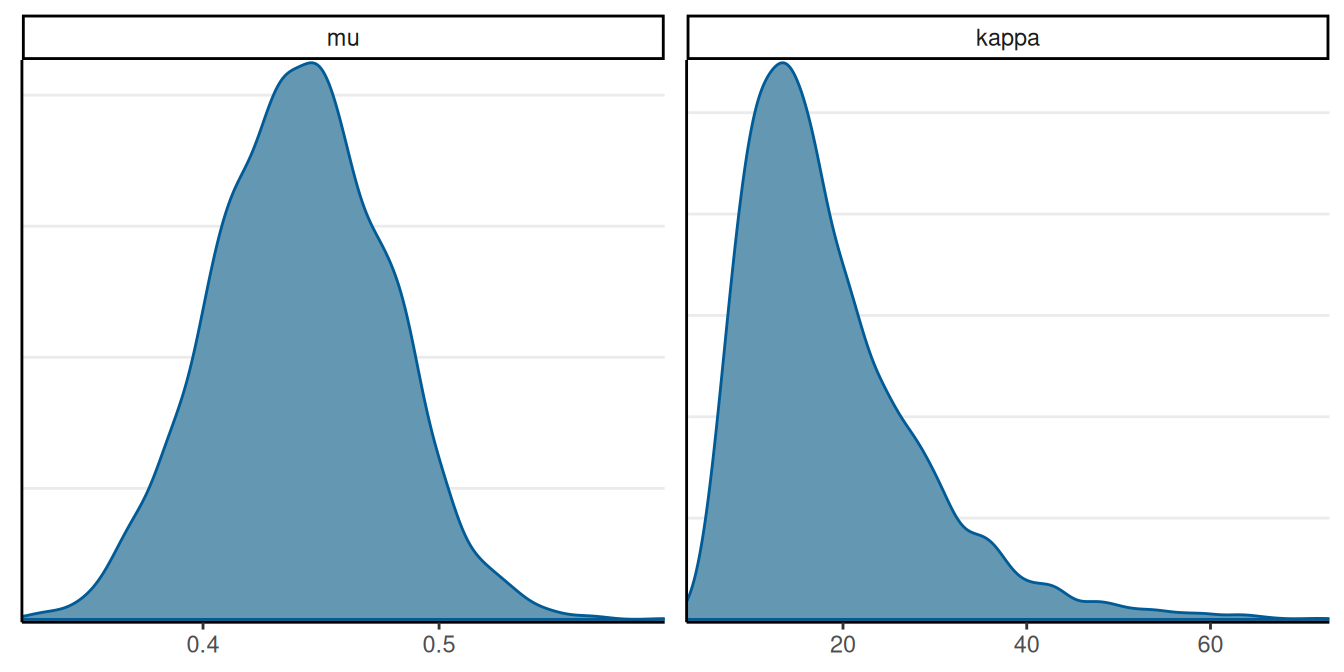
Posterior of Hyperparameters

library(bayesplot)
tt_fit$draws(c("mu", "kappa")) |>
    mcmc_dens()

The graphs show the posterior for mu and kappa. As you can see, the average probability of guessing correctly has most density between .4 and .5.

For kappa, the posterior has a pretty long tail, and the value of kappa being very large, like 100 or 200, is pretty likely. So this suggests the individuals may be pretty similar to each other.

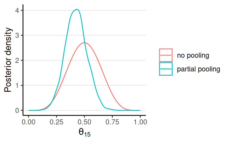
Shrinkage

From the previous model, we get posterior distributions for all parameters, including mu, kappa, and 28 thetas. The first graph shows the posterior for theta for person 1. The red curve is the one without any pooling, so the distribution is purely based on the 10 trials for person 1. The blue curve, on the other hand, is much closer to .5 due to partial pooling. Because the posterior of kappa is pretty large, the posterior is pooled towards the grand mean, mu.

For the graph below, the posterior mean is close to .5 with or without partial pooling, but the distribution is narrower with partial pooling, which reflects a stronger belief. This is because, with partial pooling, the posterior distribution uses more information than just the 10 trials of person 15; it also borrows information from the other 27 individuals.

Multiple Comparisons?

Frequentist: family-wise error rate depends on the number of intended contrasts

One advantage of the hierarchical model is it is a solution to the multiple comparison problem. In frequentist analysis, if you have multiple groups, and you want to test each contrast, you will need to consider family-wise error rate, and do something like Bonferroni corrections.

Bayesian: only one posterior; hierarchical priors already express the possibility that groups are the same

The Bayesian alternative is to do a hierarchial model with partial pooling. With Bayesian, you have one posterior distribution, which is the joint distribution of all parameters. And the use of a common distribution of the thetas already assigns some probability to the prior belief that the groups are the same.

Thus, Bayesian hierarchical model “completely solves the multiple comparisons problem.”¹

Therefore, with a hierarchical model, you can obtain the posterior of the difference of any groups, without worrying about how many comparisons you have conducted. You can read more in the sources listed here.

1. see https://statmodeling.stat.columbia.edu/2016/08/22/bayesian-inference-completely-solves-the-multiple-comparisons-problem/

Hierarchical Normal Model

In this video, we’ll talk about another Bayesian hierarchical model, the hierarchical normal model.

Effect of coaching on SAT-V

School	Treatment.Effect.Estimate	Standard.Error
A	28	15
B	8	10
C	-3	16
D	7	11
E	-1	9
F	1	11
G	18	10
H	12	18

The data come from the 1980s when scholars were debating the effect of coaching on standardized tests. The test of interest is the SAT verbal subtest. The note contains more description of it.

The analysis will be on the secondary data from eight schools, from school A to school H. Each schools conducts its own randomized trial. The middle column shows the treatment effect estimate for the effect of coaching. For example, for school A, we see that students with coaching outperformed students without coaching by 28 points. However, for schools C and E, the effects were smaller and negative.

Finally, in the last column, we have the standard error of the treatment effect for each school, based on a t-test. As you know, the smaller the standard error, the less uncertainty we have on the treatment effect.

Model: \[ \begin{aligned} d_j & \sim N(\theta_j, s_j) \\ \theta_j & \sim N(\mu, \tau) \end{aligned} \] Prior: \[ \begin{aligned} \mu & \sim N(0, 100) \\ \tau & \sim t^+_4(0, 100) \end{aligned} \]

We can use the same idea of partial pooling for this data. The idea is that, while the effect of coaching may be different across schools, there should be some similarity of the schools. Like if you are a school official, if you hear all other schools found coaching to be increasing performance, you’d probably expect coaching works for the students in your school as well.

So the logic is the same; but instead of a binomial outcome, we have something like a continuous outcome in treatment effect, so we model the treatment effect, which I call d here, by a normal distribution. Note that d here is the sample difference between the treatment and the control group; because the sample difference is not the true treatment effect, we assume d j is normally distributed with a mean theta j, where theta j is the true treatment effect for school j. s j here is the standard error of the treatment effect, the third column in the data. It reflects the degree of uncertainty in the sample treatment effect d. 

Next, we have the theta js coming from a common normal distribution, with mean mu, and standard deviation tau. So like kappa in the previous model, tau here controls how much to pool. If tau is small, it means the thetas are very similar; if tau is large, it means the thetas are very different.

data {
  int<lower=0> J;            // number of schools 
  vector[J] y;               // estimated treatment effects
  vector<lower=0>[J] sigma;  // s.e. of effect estimates 
}
parameters {
  real mu;                   // overall mean
  real<lower=0> tau;         // between-school SD
  vector[J] eta;             // standardized deviation (z score)
}
transformed parameters {
  vector[J] theta;
  theta = mu + tau * eta;    // non-centered parameterization
}
model {
  eta ~ std_normal();        // same as eta ~ normal(0, 1);
  y ~ normal(theta, sigma);
  // priors
  mu ~ normal(0, 100);
  tau ~ student_t(4, 0, 100);
}

Individual-School Treatment Effects

Prediction Interval

Posterior distribution of the true effect size of a new study, \(\tilde \theta\)

See https://onlinelibrary.wiley.com/doi/abs/10.1002/jrsm.12 for an introductory paper on random-effect meta-analysis