Introduction

PSYC 573

2024-08-27

History of Bayesian Statistics

cf. A nice popular science book by Sharon Bertsch McGrayne: The theory that would not die

Historical Figures

Thomas Bayes (1701–1762)

  • English Presbyterian minister
  • “An Essay towards solving a Problem in the Doctrine of Chances”, edited by Richard Price after Bayes’s death

Pierre-Simon Laplace (1749–1827)

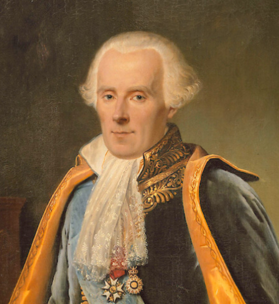
  • French Mathematician
  • Formalize Bayesian interpretation of probability, and most of the machinery for Bayesian statistics

In the 20th Century

  • Bayesian is the main way to do statistics until early 1920s

  • Ronald Fisher and Frequentist scholars took over

    “The theory of inverse probability is founded upon an error, and must be wholly rejected” (Fisher, 1925, p. 10) 1

Resurrection

  • Alan Turing’s algorithms in code breaking in World War II

  • Markov Chain Monte Carlo (MCMC) algorithms

    • Bring Bayesian back to the main stream of statistics

Why Should You Learn About the Bayesian Way?

  • Gigerenzer (2004): It is one tool of your statistical toolbox
  • Increasingly used as alternative to frequentist statistics
  • Computationally more stable for complex models
  • A coherent way of incorporating prior information
    • Common sense knowledge, previous literature, sequential experiments, etc
  • More comprehensive tools for understanding your data and models

Bayesian Ideas

Reallocation of credibility across possibilities

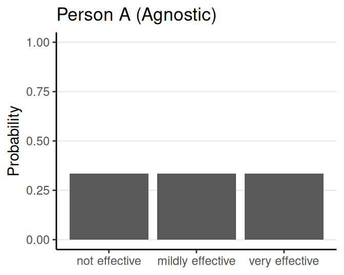
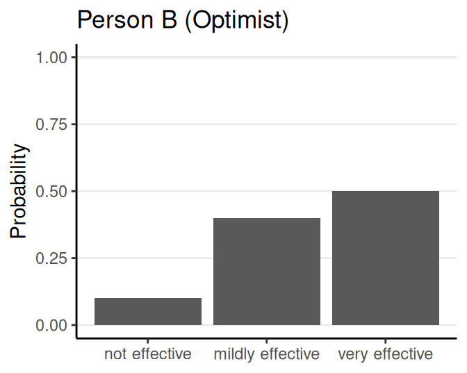
Hypothetical example: How effective is a vaccine?

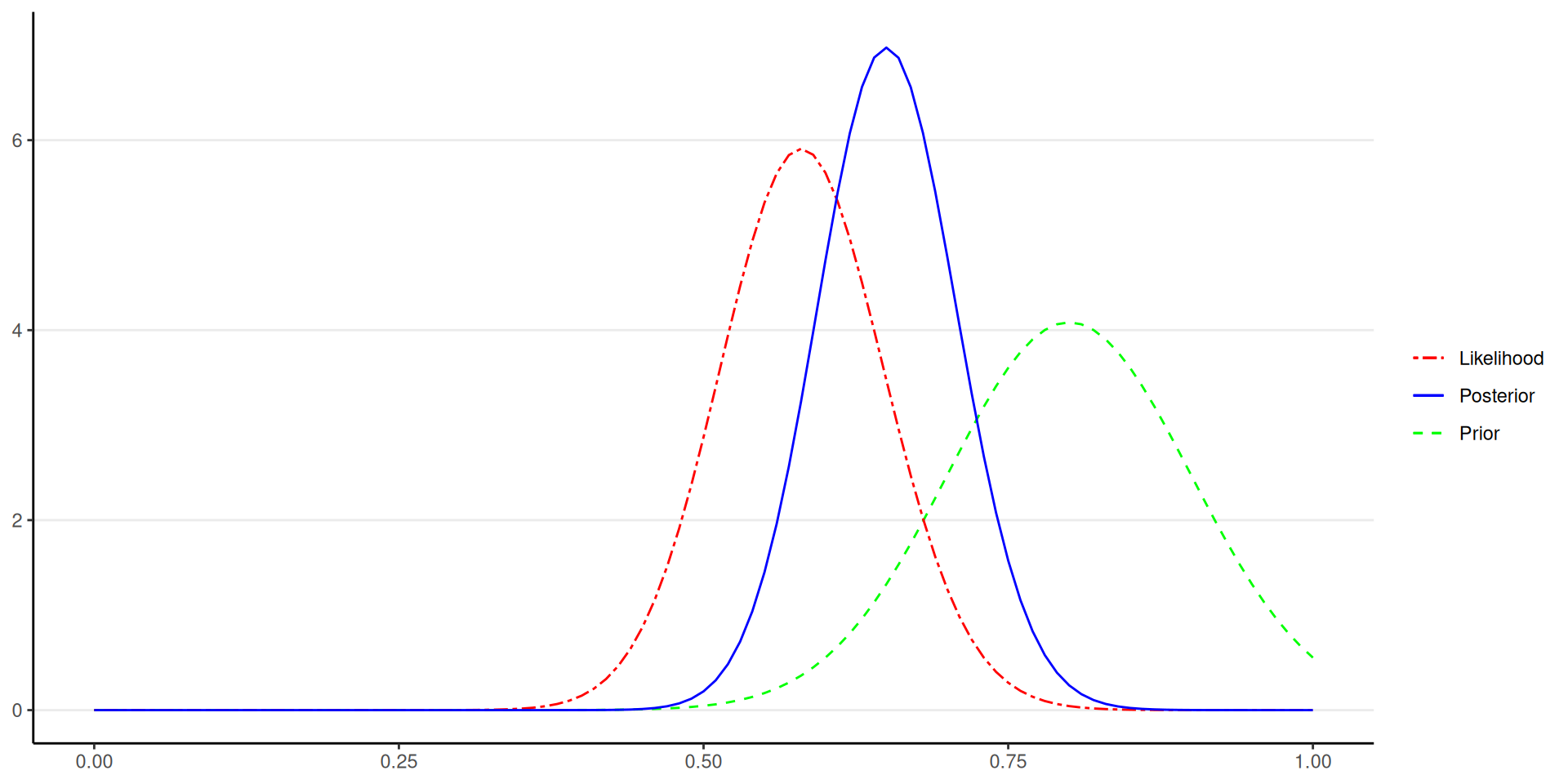
Prior (before collecting data)

Updating Beliefs

After seeing results of a trial

  • 4/5 with the vaccince improved
  • 2/5 without the vaccine improved

Possibilities = Parameter Values

A Discrete Parameter

  • Parameter: Effectiveness of the vaccine
  • Possibilities: Not effective, mildly effective, very effective

A Continuous Parameter

  • Parameter: Risk reduction by taking the vaccine
  • Possibilities: \((-\infty, \infty)\) (Any real number)

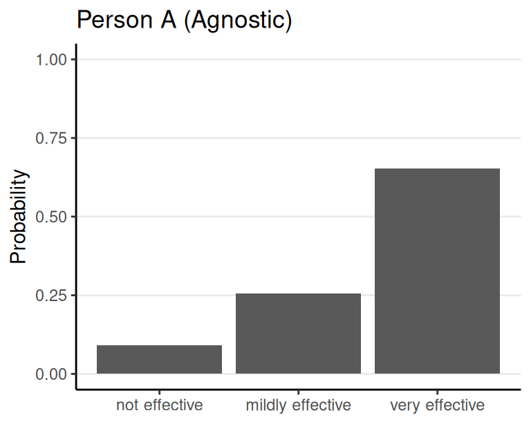
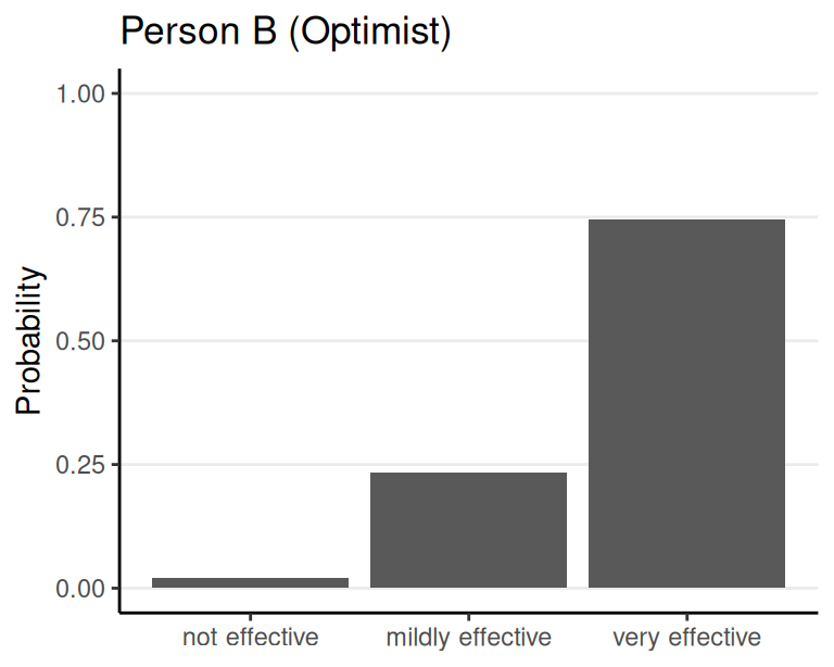
Using Bayesian analysis, one obtains updated/posterior probability for every possibility of a parameter, given the prior belief and the data

Steps of Bayesian Data Analysis

“Turning the Bayesian crank”

  1. Define a mathematical model with parameters
  2. Specify priors on parameters
  3. Check priors
  4. Fit model to data
  5. Check for convergence
  6. Evaluate the model using posterior predictive check
  7. Modify the model and repeat 3-6
  8. Obtain and interpret posterior distributions of the parameters

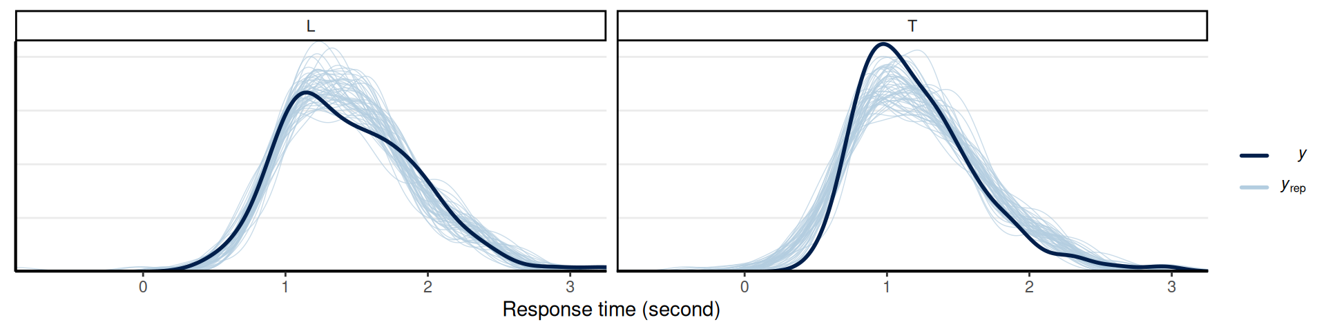
Example: Frank, Biberci, and Verschuere (2019, Cognition and Emotion)

  • Response time for 2 (Dutch–native vs. English–foreign) \(\times\) 2 (lie vs. truth) experimental conditions

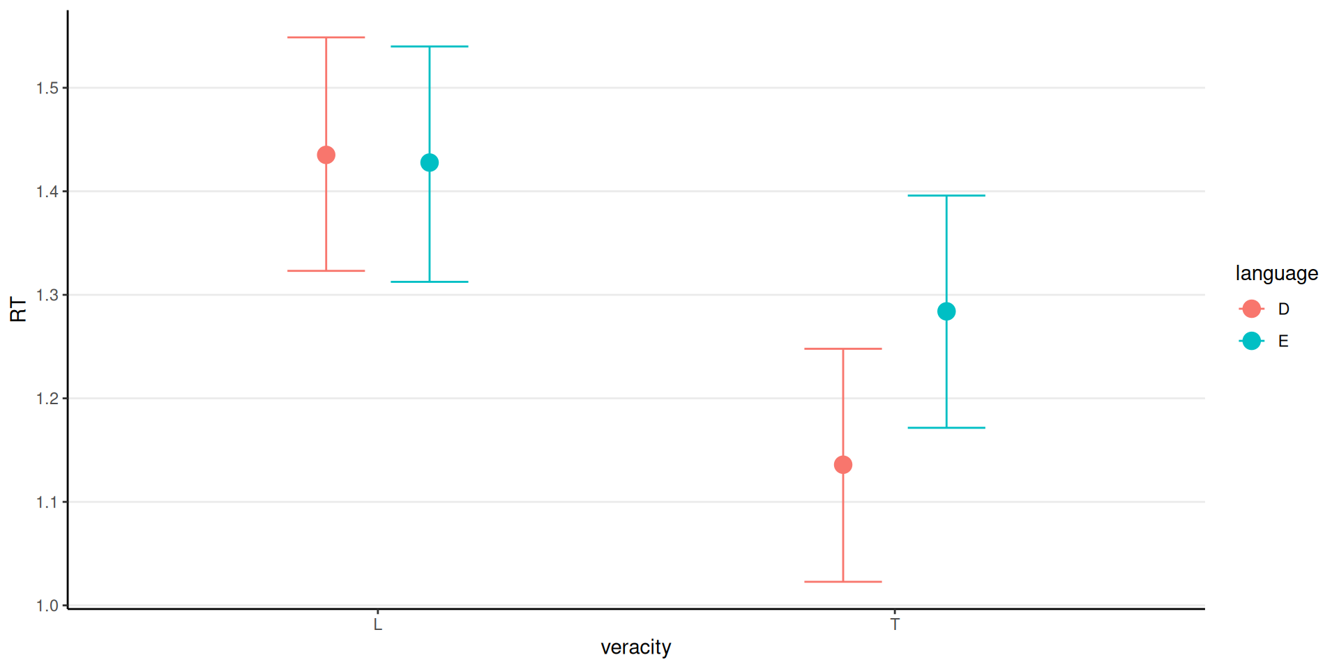
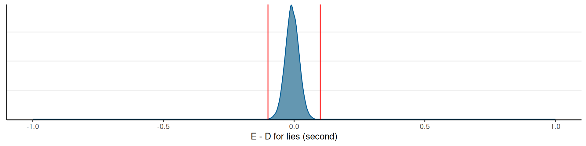
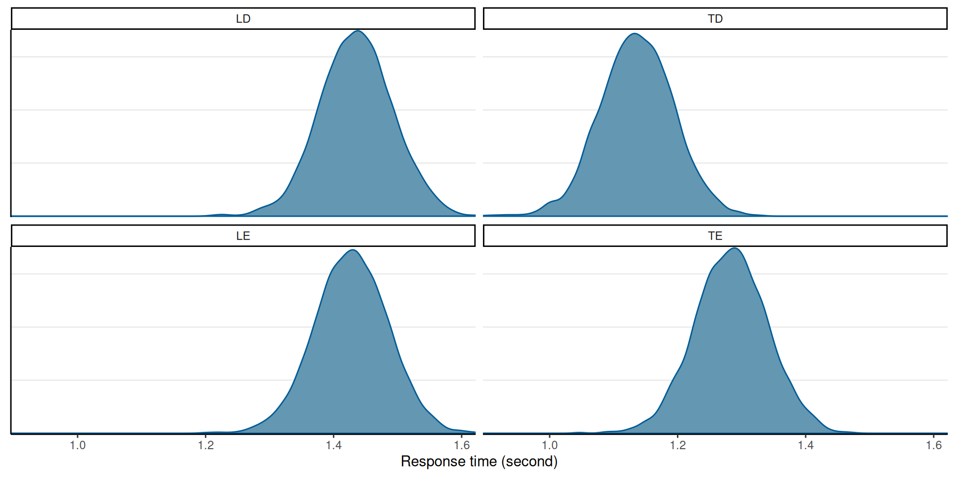
Posterior of Mean RTs by Conditions

L = Lie, T = Truth; D = Dutch, E = English

Accepting the Null

Posterior Predictive Check

Multiple Experiments

Kay, Nelson, and Hekler (2016), Figure 2

Bibliography

Frank, Avi, Sena Biberci, and Bruno Verschuere. 2019. “The Language of Lies: A Preregistered Direct Replication of Suchotzki and Gamer (2018; Experiment 2).” Cognition and Emotion 33 (6): 1310–15. https://doi.org/10.1080/02699931.2018.1553148.
Gigerenzer, Gerd. 2004. “Mindless Statistics.” The Journal of Socio-Economics 33 (5): 587–606. https://doi.org/10.1016/j.socec.2004.09.033.
Hitchcock, David B. 2003. “A History of the Metropolis–Hastings Algorithm.” The American Statistician 57 (4): 254–57. https://doi.org/10.1198/0003130032413.
Kay, Matthew, Gregory L. Nelson, and Eric B. Hekler. 2016. “Researcher-Centered Design of Statistics: Why Bayesian Statistics Better Fit the Culture and Incentives of HCI.” In Proceedings of the 2016 CHI Conference on Human Factors in Computing Systems, 4521–32. San Jose California USA: ACM. https://doi.org/10.1145/2858036.2858465.