Linear Models

PSYC 573

Statistical Model

A set of assumptions that form a simplified representation of how the data are generated

Regression

Regression

A systematic and a random components

Regression for Prediction

One outcome \(Y\), one or more predictors \(X_1\), \(X_2\), \(\ldots\)

E.g.,

What will a student’s college GPA be given an SAT score of \(x\)?
How long will a person live if the person adopts diet \(x\)?
What will the earth’s global temperature be if the carbon emission level is \(x\)?

Keep These in Mind

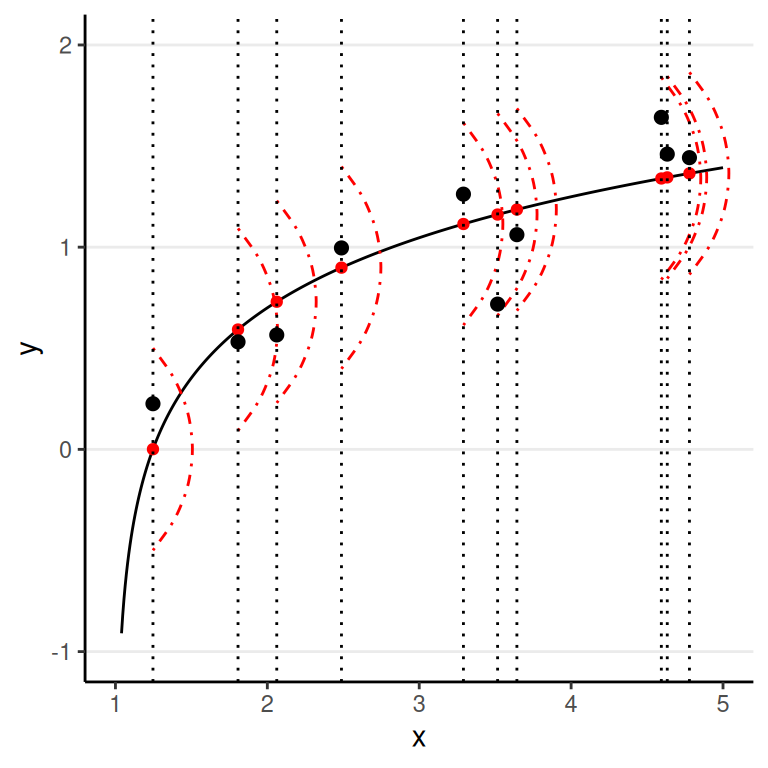
Likelihood function is defined for the outcome \(Y\)
Prediction is probabilistic (i.e., uncertain) and contains error

Linear Regression

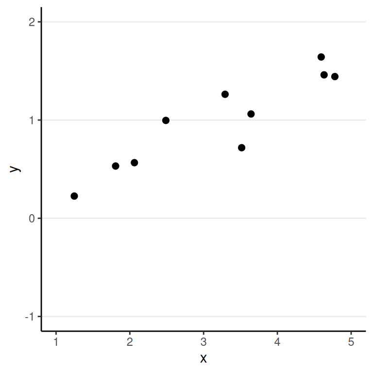
Many relations can be approximated as linear

But many relations cannot be approximated as linear

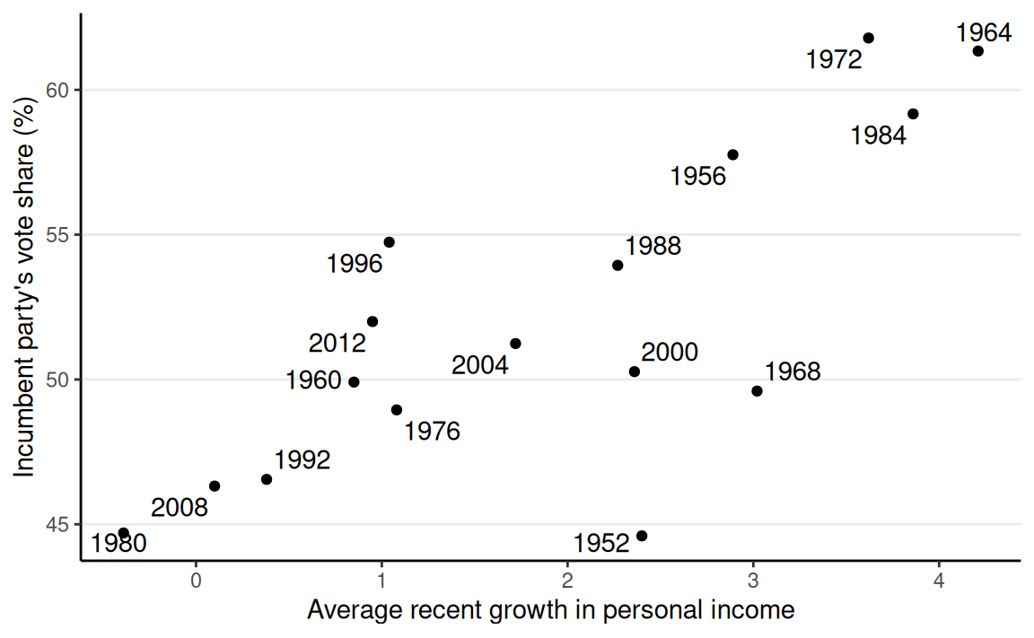
Example: “Bread and Peace” Model

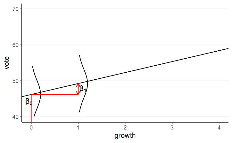
Linear Regression Model

Model:

\[ \begin{aligned} \text{vote}_i & \sim N(\mu_i, \sigma) \\ \mu_i & = \beta_0 + \beta_1 \text{growth}_i \end{aligned} \]

\(\sigma\): SD (margin) of prediction error

Prior:

\[ \begin{aligned} \beta_0 & \sim N(45, 10) \\ \beta_1 & \sim N(0, 10) \\ \sigma & \sim t^+_4(0, 5) \end{aligned} \]

Stan Code

data {
  int<lower=0> N;  // number of observations
  vector[N] y;  // outcome;
  vector[N] x;  // predictor;
  int<lower=0,upper=1> prior_only;  // whether to sample prior only
}
parameters {
  real beta0;  // regression intercept
  real beta1;  // regression coefficient
  real<lower=0> sigma;  // SD of prediction error
}
model {
  // model
  if (!prior_only) {
    y ~ normal(beta0 + beta1 * x, sigma);
  }
  // prior
  beta0 ~ normal(45, 10);
  beta1 ~ normal(0, 10);
  sigma ~ student_t(4, 0, 5);
}
generated quantities {
  // Prior/posterior predictive
  array[N] real ytilde = normal_rng(beta0 + beta1 * x, sigma);
}

Meaning of Coefficients

When growth = 0, \(\text{vote} \sim N(\beta_0, \sigma)\)

When growth = 1, \(\text{vote} \sim N(\beta_0 + \beta_1, \sigma)\)

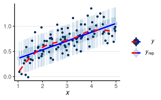
Posterior Predictive Check

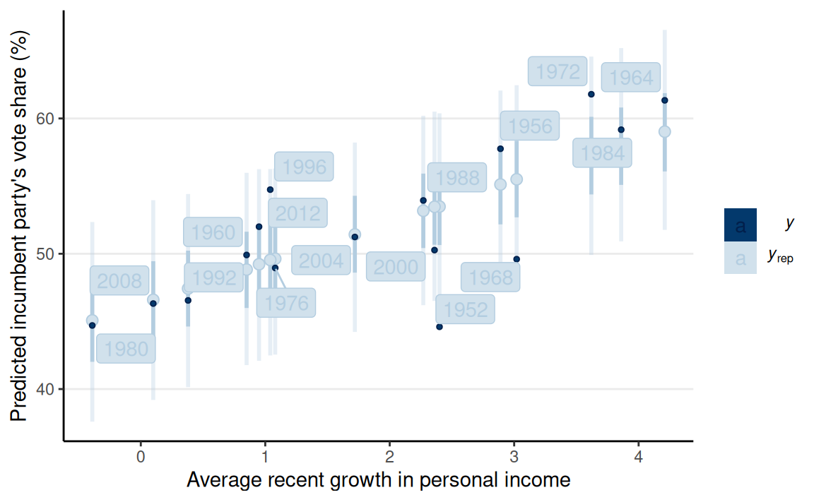
The model fits a majority of the data, but not everyone. The biggest discrepancy is 1952.

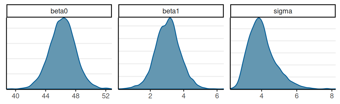
Posterior Distributions

Prediction

Predicted vote share when growth = 2: \(\tilde y \mid y \sim N(\beta_0 + \beta_1 \times 2, \sigma)\)

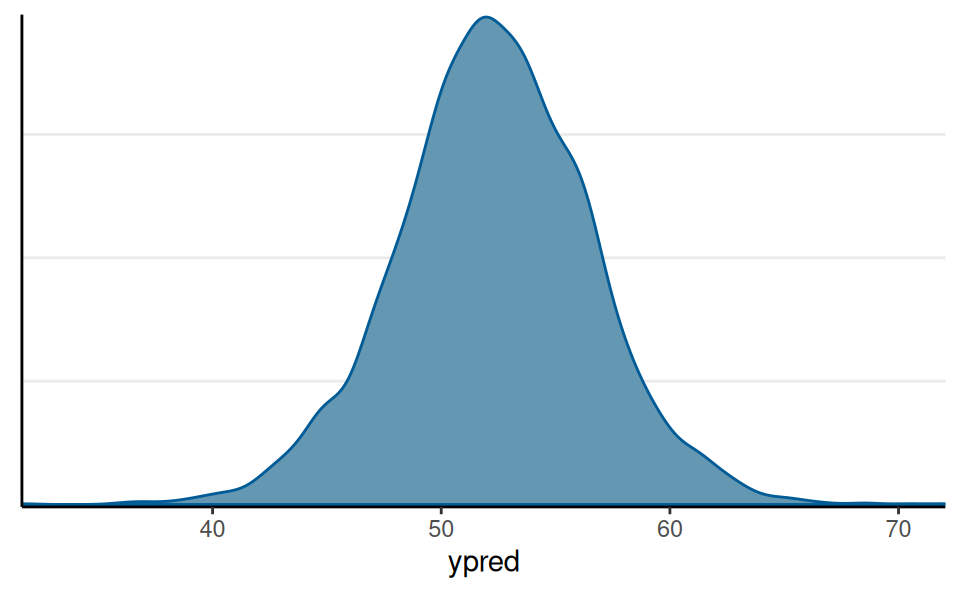
Probability of incumbent’s vote share > 50% = 0.72

Regression Diagnostics

Linearity
Independent observations
- Exchangeability in Bayesian (conditional on the predictors)
Normality
Equal variance of errors
- Same \(\sigma\) for all observations
Correct Specification of the model

Linearity (functional form)

pp_check(m_lin, type = "intervals", x = "x") +
    geom_smooth(se = FALSE, col = "blue") +
    geom_smooth(aes(x = x, y = y), se = FALSE,
                col = "red", linetype = "dashed")

Residual Plots

pp_check(m_lin_norm,
         type = "error_scatter_avg_vs_x",
         x = "x")

Multiple Predictors

Data from the 2009 American Community Survey (ACS)

Additive Model

\[ \begin{aligned} D_i & \sim N(\mu_i, \sigma) \\ \mu_i & = \beta_0 + \beta_1 S_i + \beta_2 A_i \\ \beta_0 & \sim N(0, 10) \\ \beta_1 & \sim N(0, 10) \\ \beta_2 & \sim N(0, 1) \\ \sigma & \sim t^+_4(0, 3) \end{aligned} \]

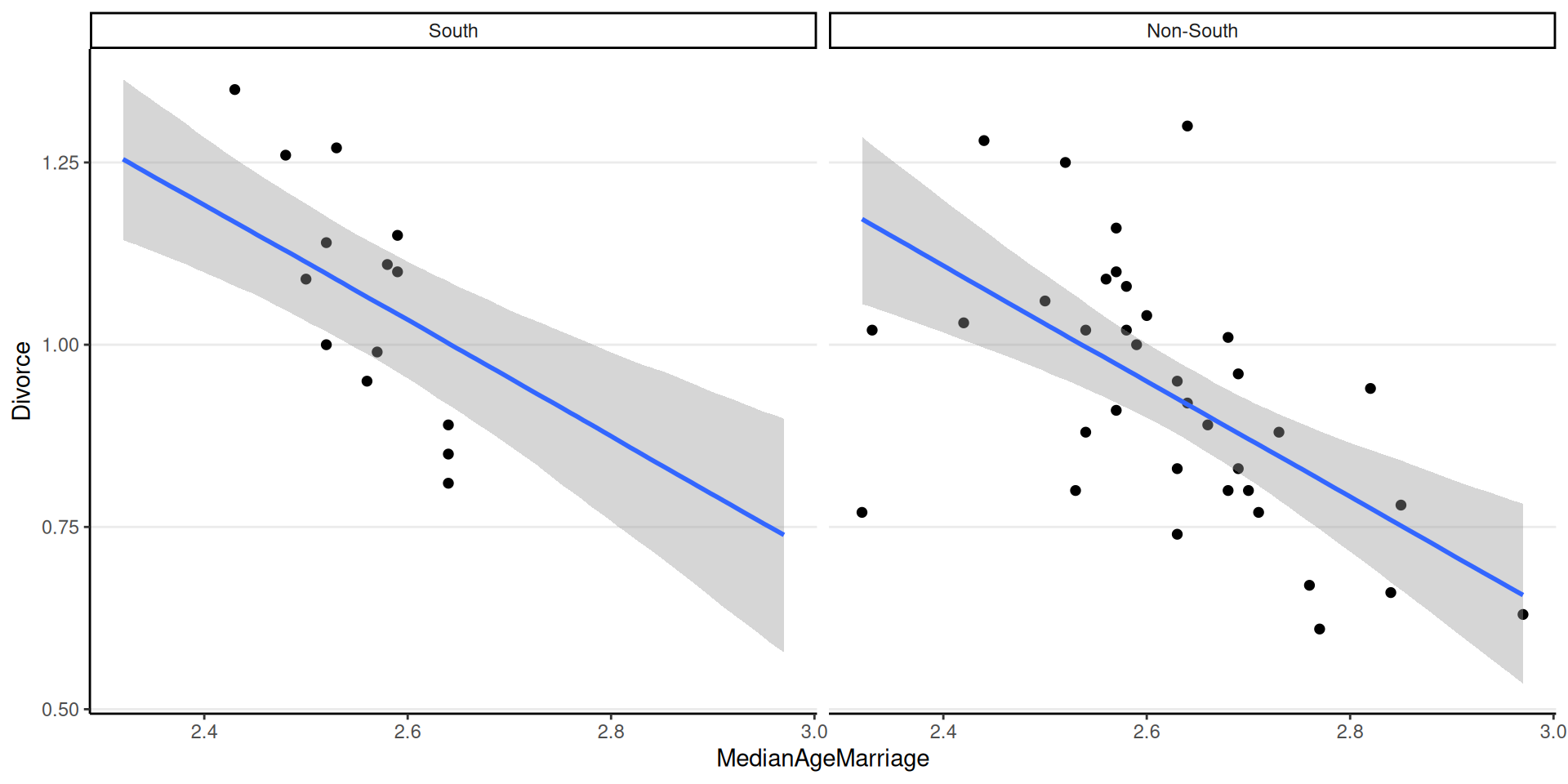
\(\beta_1\): Expected difference in divorce rate between southern and non-southern states with the same median age of marriage.
\(\beta_2\): Expected difference in divorce rate for one unit difference in median age of marriage, when both states are southern (or non-southern).

The `brms` R package

library(brms)
options(brms.backend = "cmdstanr")  # use cmdstanr instead of rstan
get_prior(Divorce ~ MedianAgeMarriage + South,
          data = waffle_divorce)

                prior     class              coef group resp dpar nlpar lb ub
               (flat)         b                                              
               (flat)         b MedianAgeMarriage                            
               (flat)         b        Southsouth                            
 student_t(3, 1, 2.5) Intercept                                              
 student_t(3, 0, 2.5)     sigma                                          0   
       source
      default
 (vectorized)
 (vectorized)
      default
      default

Beware of the default priors

Please note that the default priors could change in future versions of the brms package. It has changed in previous releases.

m_additive <- brm(
1    Divorce ~ South + MedianAgeMarriage,
    data = waffle_divorce,
2    prior = prior(normal(0, 2), class = "b") +
        prior(normal(0, 10), class = "b", coef = "Southsouth") +
        prior(normal(0, 10), class = "Intercept") +
        prior(student_t(4, 0, 3), class = "sigma"),
3    seed = 941,
4    file = "m_additive"
)
summary(m_additive)

1: Same formula syntax as in lm().
2: Prior distributions (class = b for \(\beta\) coefficients, sigma for the \(\sigma\) parameter)
3: For reproducibility
4: Save results to m_additive.rds

Running MCMC with 4 sequential chains...

Chain 1 Iteration:    1 / 2000 [  0%]  (Warmup) 
Chain 1 Iteration:  100 / 2000 [  5%]  (Warmup) 
Chain 1 Iteration:  200 / 2000 [ 10%]  (Warmup) 
Chain 1 Iteration:  300 / 2000 [ 15%]  (Warmup) 
Chain 1 Iteration:  400 / 2000 [ 20%]  (Warmup) 
Chain 1 Iteration:  500 / 2000 [ 25%]  (Warmup) 
Chain 1 Iteration:  600 / 2000 [ 30%]  (Warmup) 
Chain 1 Iteration:  700 / 2000 [ 35%]  (Warmup) 
Chain 1 Iteration:  800 / 2000 [ 40%]  (Warmup) 
Chain 1 Iteration:  900 / 2000 [ 45%]  (Warmup) 
Chain 1 Iteration: 1000 / 2000 [ 50%]  (Warmup) 
Chain 1 Iteration: 1001 / 2000 [ 50%]  (Sampling) 
Chain 1 Iteration: 1100 / 2000 [ 55%]  (Sampling) 
Chain 1 Iteration: 1200 / 2000 [ 60%]  (Sampling) 
Chain 1 Iteration: 1300 / 2000 [ 65%]  (Sampling) 
Chain 1 Iteration: 1400 / 2000 [ 70%]  (Sampling) 
Chain 1 Iteration: 1500 / 2000 [ 75%]  (Sampling) 
Chain 1 Iteration: 1600 / 2000 [ 80%]  (Sampling) 
Chain 1 Iteration: 1700 / 2000 [ 85%]  (Sampling) 
Chain 1 Iteration: 1800 / 2000 [ 90%]  (Sampling) 
Chain 1 Iteration: 1900 / 2000 [ 95%]  (Sampling) 
Chain 1 Iteration: 2000 / 2000 [100%]  (Sampling) 
Chain 1 finished in 0.0 seconds.
Chain 2 Iteration:    1 / 2000 [  0%]  (Warmup) 
Chain 2 Iteration:  100 / 2000 [  5%]  (Warmup) 
Chain 2 Iteration:  200 / 2000 [ 10%]  (Warmup) 
Chain 2 Iteration:  300 / 2000 [ 15%]  (Warmup) 
Chain 2 Iteration:  400 / 2000 [ 20%]  (Warmup) 
Chain 2 Iteration:  500 / 2000 [ 25%]  (Warmup) 
Chain 2 Iteration:  600 / 2000 [ 30%]  (Warmup) 
Chain 2 Iteration:  700 / 2000 [ 35%]  (Warmup) 
Chain 2 Iteration:  800 / 2000 [ 40%]  (Warmup) 
Chain 2 Iteration:  900 / 2000 [ 45%]  (Warmup) 
Chain 2 Iteration: 1000 / 2000 [ 50%]  (Warmup) 
Chain 2 Iteration: 1001 / 2000 [ 50%]  (Sampling) 
Chain 2 Iteration: 1100 / 2000 [ 55%]  (Sampling) 
Chain 2 Iteration: 1200 / 2000 [ 60%]  (Sampling) 
Chain 2 Iteration: 1300 / 2000 [ 65%]  (Sampling) 
Chain 2 Iteration: 1400 / 2000 [ 70%]  (Sampling) 
Chain 2 Iteration: 1500 / 2000 [ 75%]  (Sampling) 
Chain 2 Iteration: 1600 / 2000 [ 80%]  (Sampling) 
Chain 2 Iteration: 1700 / 2000 [ 85%]  (Sampling) 
Chain 2 Iteration: 1800 / 2000 [ 90%]  (Sampling) 
Chain 2 Iteration: 1900 / 2000 [ 95%]  (Sampling) 
Chain 2 Iteration: 2000 / 2000 [100%]  (Sampling) 
Chain 2 finished in 0.0 seconds.
Chain 3 Iteration:    1 / 2000 [  0%]  (Warmup) 
Chain 3 Iteration:  100 / 2000 [  5%]  (Warmup) 
Chain 3 Iteration:  200 / 2000 [ 10%]  (Warmup) 
Chain 3 Iteration:  300 / 2000 [ 15%]  (Warmup) 
Chain 3 Iteration:  400 / 2000 [ 20%]  (Warmup) 
Chain 3 Iteration:  500 / 2000 [ 25%]  (Warmup) 
Chain 3 Iteration:  600 / 2000 [ 30%]  (Warmup) 
Chain 3 Iteration:  700 / 2000 [ 35%]  (Warmup) 
Chain 3 Iteration:  800 / 2000 [ 40%]  (Warmup) 
Chain 3 Iteration:  900 / 2000 [ 45%]  (Warmup) 
Chain 3 Iteration: 1000 / 2000 [ 50%]  (Warmup) 
Chain 3 Iteration: 1001 / 2000 [ 50%]  (Sampling) 
Chain 3 Iteration: 1100 / 2000 [ 55%]  (Sampling) 
Chain 3 Iteration: 1200 / 2000 [ 60%]  (Sampling) 
Chain 3 Iteration: 1300 / 2000 [ 65%]  (Sampling) 
Chain 3 Iteration: 1400 / 2000 [ 70%]  (Sampling) 
Chain 3 Iteration: 1500 / 2000 [ 75%]  (Sampling) 
Chain 3 Iteration: 1600 / 2000 [ 80%]  (Sampling) 
Chain 3 Iteration: 1700 / 2000 [ 85%]  (Sampling) 
Chain 3 Iteration: 1800 / 2000 [ 90%]  (Sampling) 
Chain 3 Iteration: 1900 / 2000 [ 95%]  (Sampling) 
Chain 3 Iteration: 2000 / 2000 [100%]  (Sampling) 
Chain 3 finished in 0.0 seconds.
Chain 4 Iteration:    1 / 2000 [  0%]  (Warmup) 
Chain 4 Iteration:  100 / 2000 [  5%]  (Warmup) 
Chain 4 Iteration:  200 / 2000 [ 10%]  (Warmup) 
Chain 4 Iteration:  300 / 2000 [ 15%]  (Warmup) 
Chain 4 Iteration:  400 / 2000 [ 20%]  (Warmup) 
Chain 4 Iteration:  500 / 2000 [ 25%]  (Warmup) 
Chain 4 Iteration:  600 / 2000 [ 30%]  (Warmup) 
Chain 4 Iteration:  700 / 2000 [ 35%]  (Warmup) 
Chain 4 Iteration:  800 / 2000 [ 40%]  (Warmup) 
Chain 4 Iteration:  900 / 2000 [ 45%]  (Warmup) 
Chain 4 Iteration: 1000 / 2000 [ 50%]  (Warmup) 
Chain 4 Iteration: 1001 / 2000 [ 50%]  (Sampling) 
Chain 4 Iteration: 1100 / 2000 [ 55%]  (Sampling) 
Chain 4 Iteration: 1200 / 2000 [ 60%]  (Sampling) 
Chain 4 Iteration: 1300 / 2000 [ 65%]  (Sampling) 
Chain 4 Iteration: 1400 / 2000 [ 70%]  (Sampling) 
Chain 4 Iteration: 1500 / 2000 [ 75%]  (Sampling) 
Chain 4 Iteration: 1600 / 2000 [ 80%]  (Sampling) 
Chain 4 Iteration: 1700 / 2000 [ 85%]  (Sampling) 
Chain 4 Iteration: 1800 / 2000 [ 90%]  (Sampling) 
Chain 4 Iteration: 1900 / 2000 [ 95%]  (Sampling) 
Chain 4 Iteration: 2000 / 2000 [100%]  (Sampling) 
Chain 4 finished in 0.0 seconds.

All 4 chains finished successfully.
Mean chain execution time: 0.0 seconds.
Total execution time: 0.6 seconds.

 Family: gaussian 
  Links: mu = identity; sigma = identity 
Formula: Divorce ~ South + MedianAgeMarriage 
   Data: waffle_divorce (Number of observations: 50) 
  Draws: 4 chains, each with iter = 2000; warmup = 1000; thin = 1;
         total post-warmup draws = 4000

Regression Coefficients:
                  Estimate Est.Error l-95% CI u-95% CI Rhat Bulk_ESS Tail_ESS
Intercept             3.01      0.45     2.12     3.89 1.00     3949     2957
Southsouth            0.08      0.05    -0.01     0.18 1.00     3943     2798
MedianAgeMarriage    -0.79      0.17    -1.13    -0.45 1.00     3947     2918

Further Distributional Parameters:
      Estimate Est.Error l-95% CI u-95% CI Rhat Bulk_ESS Tail_ESS
sigma     0.15      0.02     0.12     0.18 1.00     3284     2523

Draws were sampled using sample(hmc). For each parameter, Bulk_ESS
and Tail_ESS are effective sample size measures, and Rhat is the potential
scale reduction factor on split chains (at convergence, Rhat = 1).

Slopes are parallel

Interactions

\[ \begin{aligned} D_i & \sim N(\mu_i, \sigma) \\ \mu_i & = \beta_0 + \beta_1 S_i + \beta_2 A_i + \beta_3 S_i \times A_i \\ \beta_0, \beta_1 & \sim N(0, 10) \\ \beta_2 & \sim N(0, 1) \\ \beta_3 & \sim N(0, 2) \\ \sigma & \sim t^+_4(0, 3) \end{aligned} \]

\(\beta_1\): Difference in intercept between southern and non-southern states.
\(\beta_3\): Difference in the coefficient for A → D between southern and non-southern states

\(\beta_1\) and \(\beta_2\) Are Not Main Effects

When an interaction term is included, the coefficient of \(A\) is the conditional effect when \(S\) = 0.

Reporting I

We fit a Bayesian linear model using the brms R package to examine the interaction effects between state-level median age of marriage and location of the state (southern vs. non-southern). We use weakly informative priors for all model parameters, as shown below: [insert the model equations]

Reporting II

The posterior distributions are obtained using Markov Chain Monte Carlo (MCMC) sampling, with 4 chains and 2,000 iterations for each chain (the first 1,000 discarded as warm-ups). Convergence of MCMC chains were determined by examining trace plots of the posterior samples and the \(\hat R\) statistics (< 1.01 for all model parameters; Vehtari et al., 2021), and the effective sample sizes are > 400 to ensure accurate approximation of the posterior distributions.

 Family: gaussian 
  Links: mu = identity; sigma = identity 
Formula: Divorce ~ South * MedianAgeMarriage 
   Data: waffle_divorce (Number of observations: 50) 
  Draws: 4 chains, each with iter = 4000; warmup = 2000; thin = 1;
         total post-warmup draws = 8000

Regression Coefficients:
                             Estimate Est.Error l-95% CI u-95% CI Rhat Bulk_ESS
Intercept                        2.78      0.46     1.87     3.68 1.00     4716
Southsouth                       3.20      1.60     0.19     6.30 1.00     2863
MedianAgeMarriage               -0.70      0.18    -1.05    -0.35 1.00     4714
Southsouth:MedianAgeMarriage    -1.22      0.62    -2.42    -0.03 1.00     2876
                             Tail_ESS
Intercept                        4042
Southsouth                       3608
MedianAgeMarriage                4085
Southsouth:MedianAgeMarriage     3584

Further Distributional Parameters:
      Estimate Est.Error l-95% CI u-95% CI Rhat Bulk_ESS Tail_ESS
sigma     0.14      0.02     0.12     0.18 1.00     4244     4998

Draws were sampled using sample(hmc). For each parameter, Bulk_ESS
and Tail_ESS are effective sample size measures, and Rhat is the potential
scale reduction factor on split chains (at convergence, Rhat = 1).

Simple Slopes/Conditional Effects

Slope when South = 0: \(\beta_1\)
Slope when South = 1: \(\beta_1 + \beta_3\)

variable	mean	median	sd	mad	q5	q95	rhat	ess_bulk	ess_tail
b_nonsouth	-0.70	-0.71	0.18	0.18	-1.00	-0.41	1	4714	4085
b_south	-1.92	-1.91	0.60	0.60	-2.91	-0.93	1	3168	3659

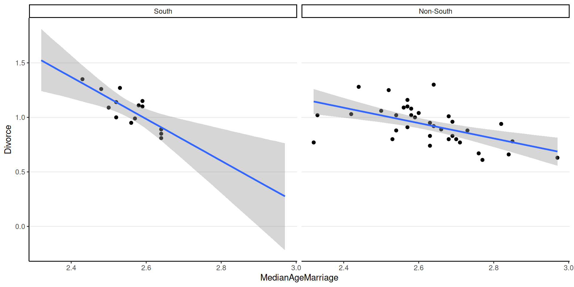
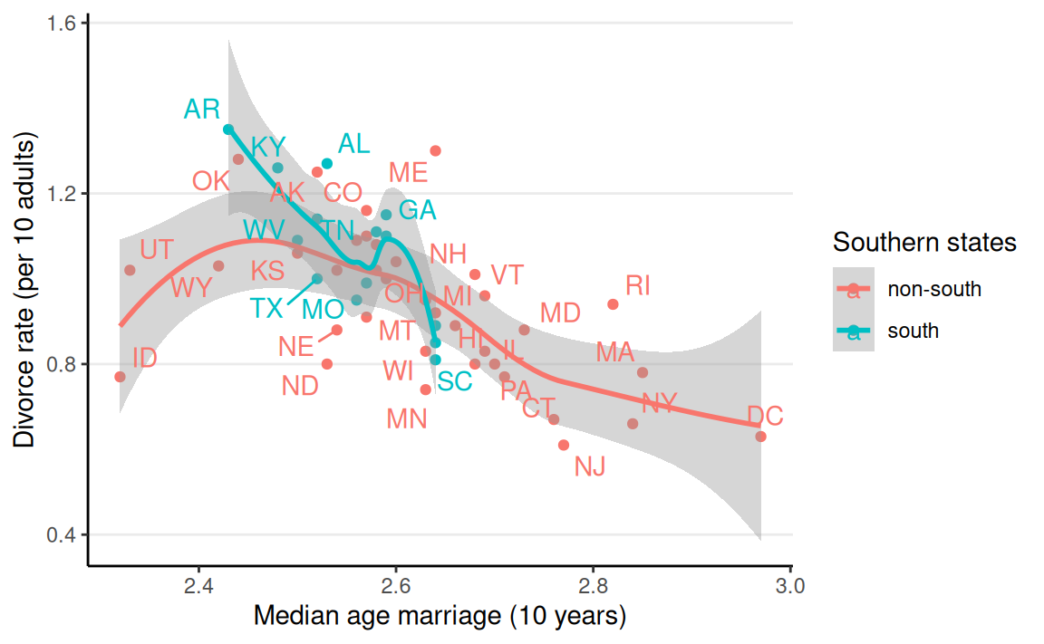
Figure 1: Model-implied simple slopes based on the interaction model (posterior median and 95% symmetric credible band).

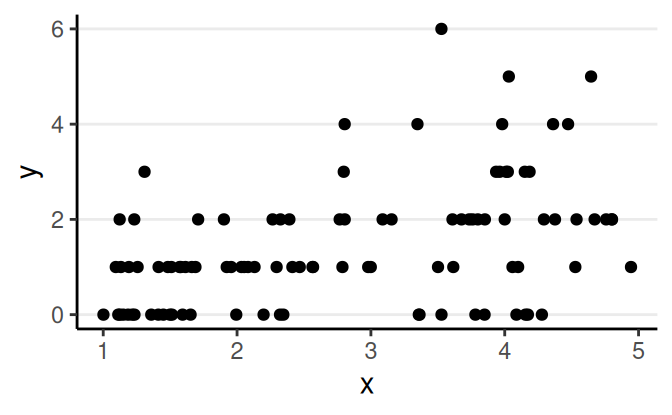
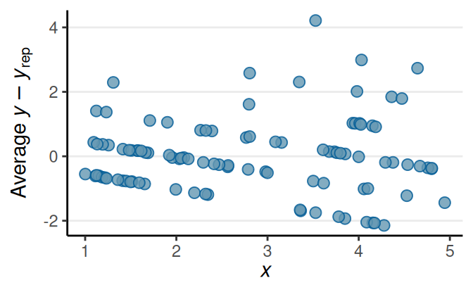
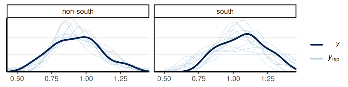
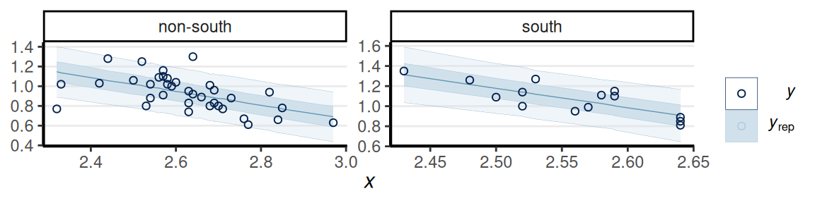
Posterior Predictive Checks

Reporting III

As shown in Figure 1, median age of marriage negatively predicts divorce rate in both southern and non-southern states. For non-southern states, a 10-year difference in median age of marriage corresponds to a difference of -0.7 per 10 adults, 95% CI [-1.05, -0.35] in divorce rate. There is evidence for a nonzero interaction effect such that the negative association between median age of marriage and divorce rate in southern states is stronger than in non-southern states, \(\beta_3\) = -1.22, 95% CI [-2.42, -0.03].

Centering

Intercept (\(\beta_0\)): Predicted \(y\) when all predictors are 0

i.e., non-southern states with median marriage age of 0.

To make \(\beta_0\) more meaningful, center the predictors at a more meaningful value.

The Intercept below shows the predicted divorce rate with a median age of marriage of 25. \(\beta_1\) represents the difference between southern and non-southern states conditional on median marriage age of 25.

 Family: gaussian 
  Links: mu = identity; sigma = identity 
Formula: Divorce ~ South * I(MedianAgeMarriage - 2.5) 
   Data: waffle_divorce (Number of observations: 50) 
  Draws: 4 chains, each with iter = 4000; warmup = 2000; thin = 1;
         total post-warmup draws = 8000

Regression Coefficients:
                                  Estimate Est.Error l-95% CI u-95% CI Rhat
Intercept                             1.02      0.03     0.95     1.08 1.00
Southsouth                            0.16      0.06     0.04     0.28 1.00
IMedianAgeMarriageM2.5               -0.70      0.18    -1.06    -0.35 1.00
Southsouth:IMedianAgeMarriageM2.5    -1.24      0.61    -2.42    -0.06 1.00
                                  Bulk_ESS Tail_ESS
Intercept                             7332     5420
Southsouth                            5730     5778
IMedianAgeMarriageM2.5                7481     5345
Southsouth:IMedianAgeMarriageM2.5     6276     6331

Further Distributional Parameters:
      Estimate Est.Error l-95% CI u-95% CI Rhat Bulk_ESS Tail_ESS
sigma     0.14      0.02     0.12     0.18 1.00     7285     5539

Draws were sampled using sample(hmc). For each parameter, Bulk_ESS
and Tail_ESS are effective sample size measures, and Rhat is the potential
scale reduction factor on split chains (at convergence, Rhat = 1).

Linear Models

Statistical Model

Regression

Regression

Regression for Prediction

Keep These in Mind

Linear Regression

Example: “Bread and Peace” Model

Linear Regression Model

Stan Code

Meaning of Coefficients

Posterior Predictive Check

Posterior Distributions

Prediction

Regression Diagnostics

Linearity (functional form)

Residual Plots

Multiple Predictors

Additive Model

The brms R package

Interactions

Reporting I

Reporting II

Simple Slopes/Conditional Effects

Posterior Predictive Checks

Reporting III

Centering

The `brms` R package