Markov Chain Monte Carlo
PSYC 573
Monte Carlo (MC) Methods

- 1930s and 40s: answer questions in nuclear physics not solvable with conventional mathematical methods
- Key figures: Stanislaw Ulam, John von Neumann, Nicholas Metropolis
- Central element of the Manhattan Project in the development of the hydrogen bomb
MC With One Unknown
rbeta(), rnorm(), rbinom(): generate values that imitate independent samples from known distributions
- use pseudorandom numbers
E.g., rbeta(n, shape1 = 15, shape2 = 10)
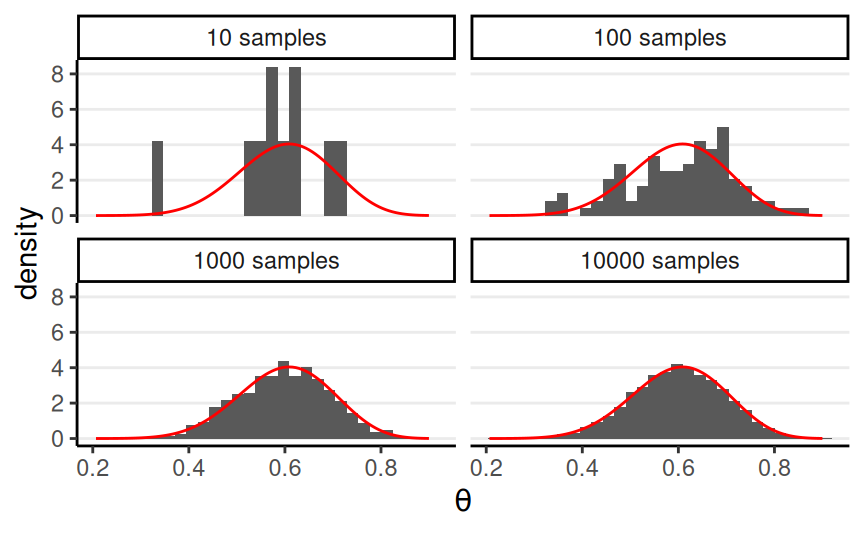
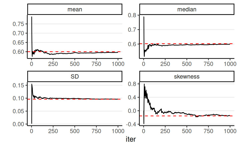
With a large number of draws (S),
- sample density \(\to\) target distribution
- most sample statistics (e.g., mean, quantiles) \(\to\) corresponding characteristics of the target density
An Analogy

You have a task: tour all regions in LA county, and the time your spend on each region should be proportional to its popularity
However, you don’t know which region is the most popular
Each day, you will decide whether to stay in the current region or move to a neighboring region
You have a tour guide that tells you whether region A is more or less popular than region B and by how much
How would you proceed?
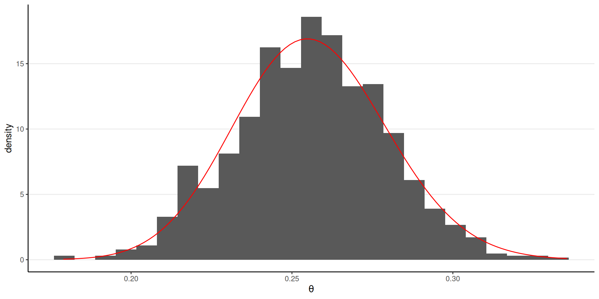
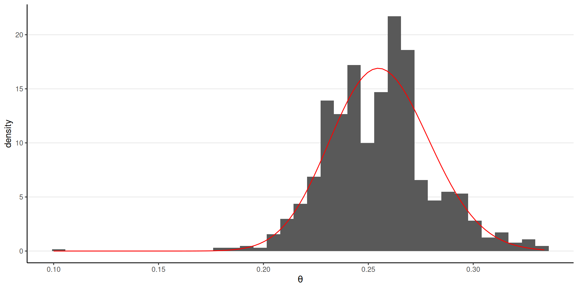
Analytic Posterior
Beta(1.5, 2) prior \(\to\) Beta(87.5, 254) posterior
1,000 independent draws from the posterior:
With the Metropolis Algorithm
Proposal density: \(N(0, 0.1)\); Starting value: \(\theta^{(1)} = 0.1\)
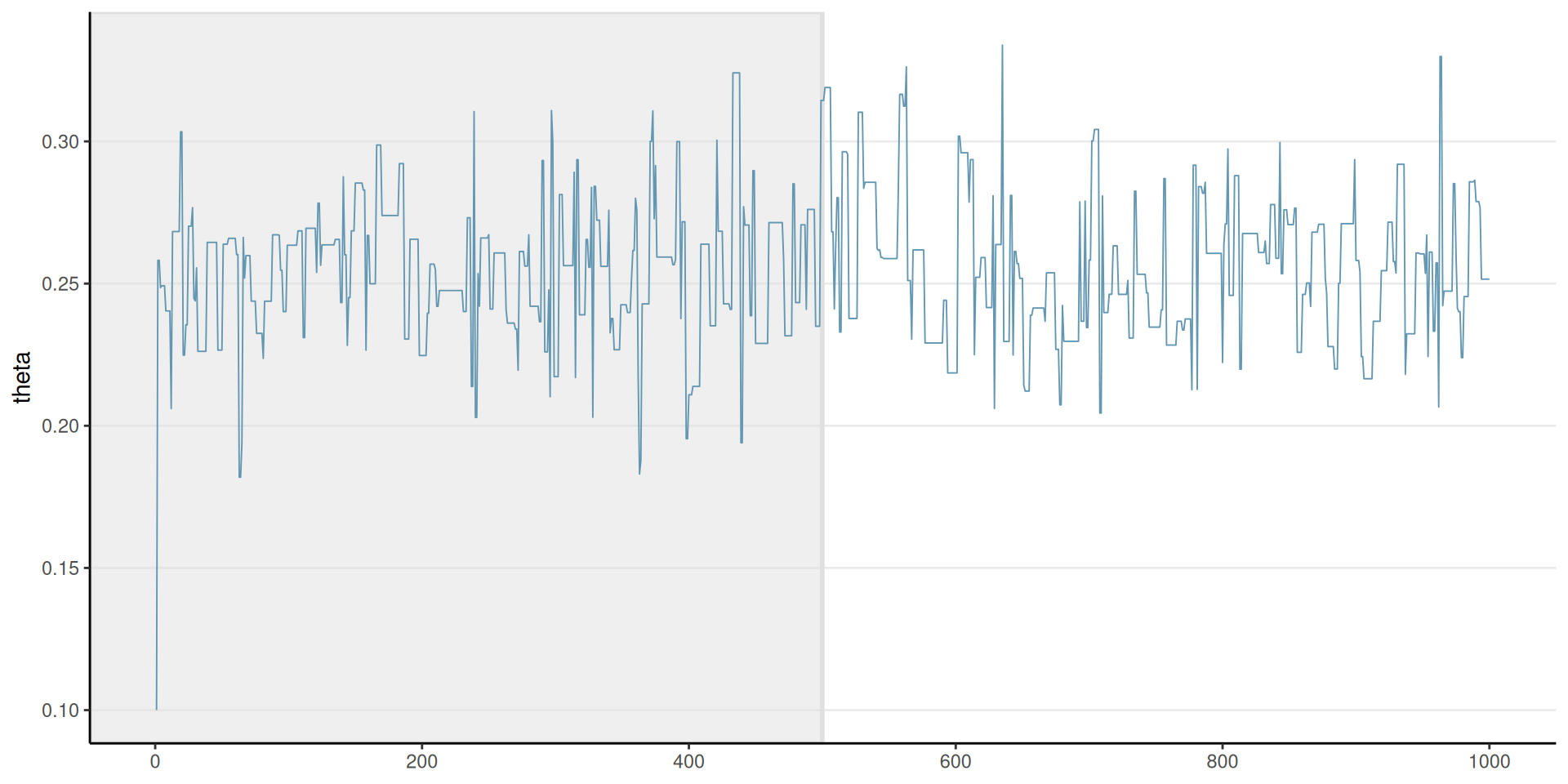
Warm-up
It takes a few to a few hundred thousand iterations for the chain to get to the stationary distribution
Therefore, a common practice is to discard the first \(S_\text{warm-up}\) (e.g., first half of the) iterations
- Also called burn-in
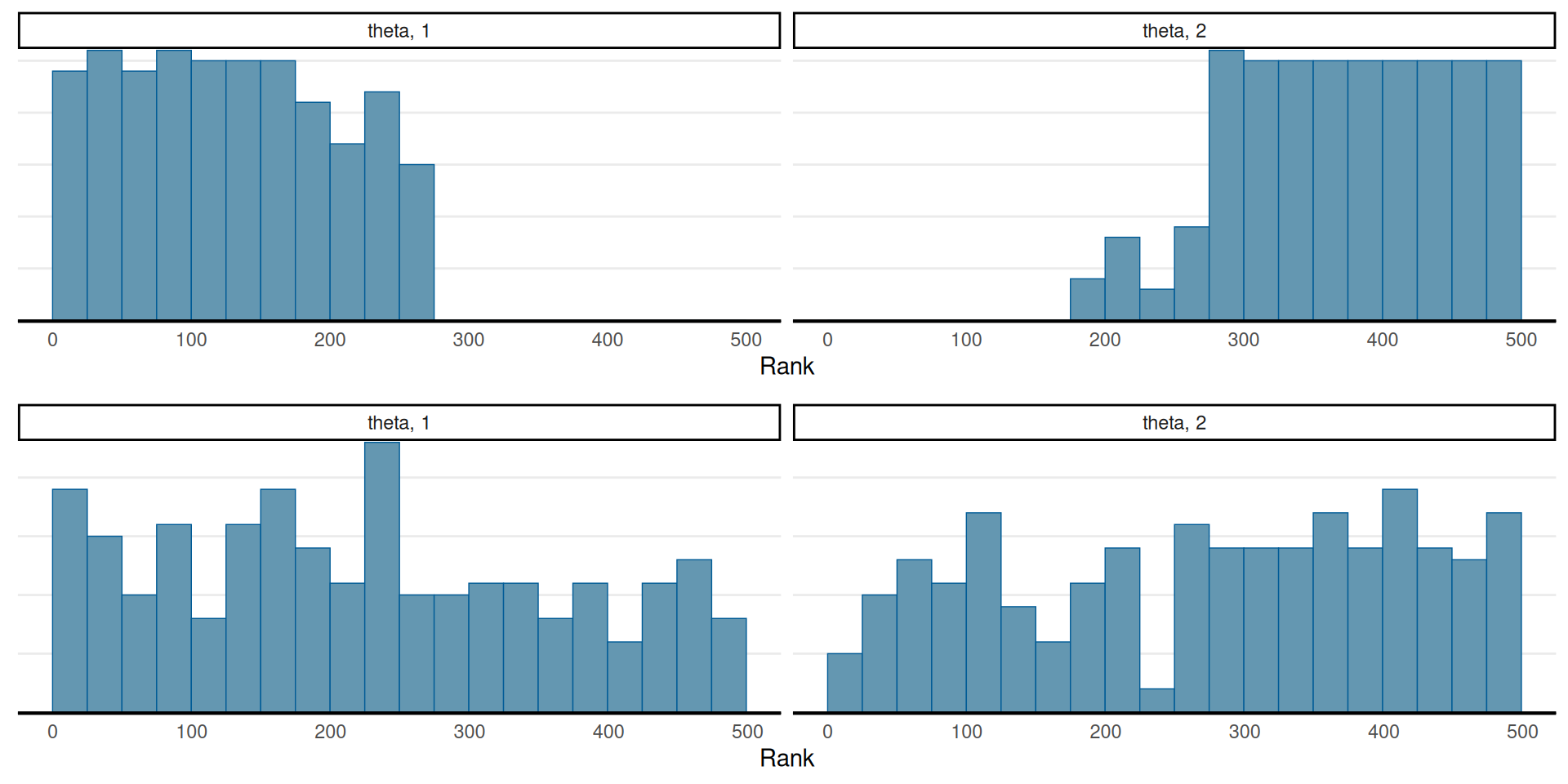
Representativeness
The chain does not get stuck
Mixing: multiple chains cross each other
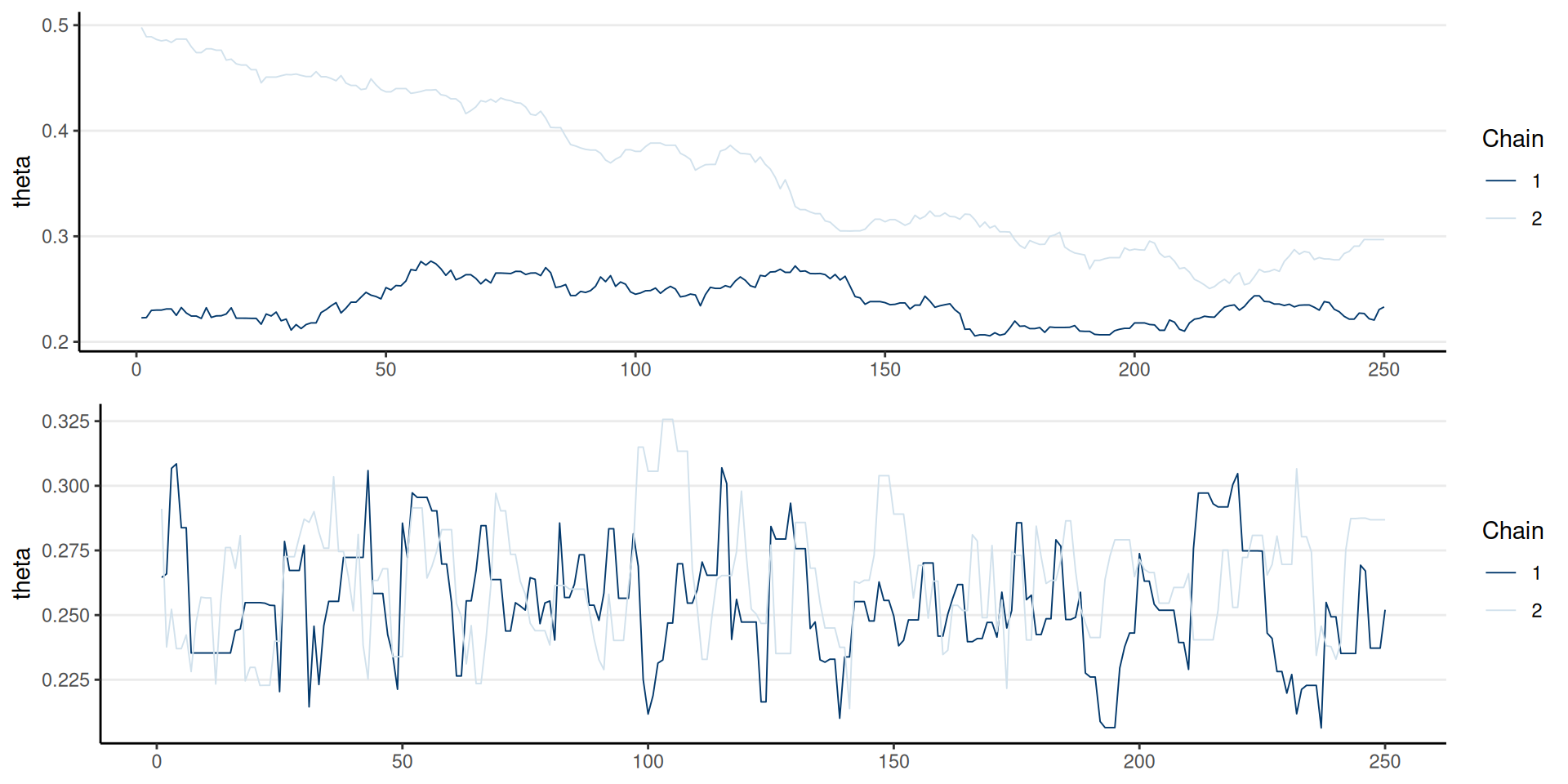
Representativeness (cont’d)
For more robust diagnostics (Vehtari et al. 2021)
- The rank histograms should look like uniform distributions