  Reaction Days Subject
1      250    0     308
2      259    1     308
3      251    2     308
4      321    3     308
5      357    4     308
6 415 5 308Multilevel Models
PSYC 573
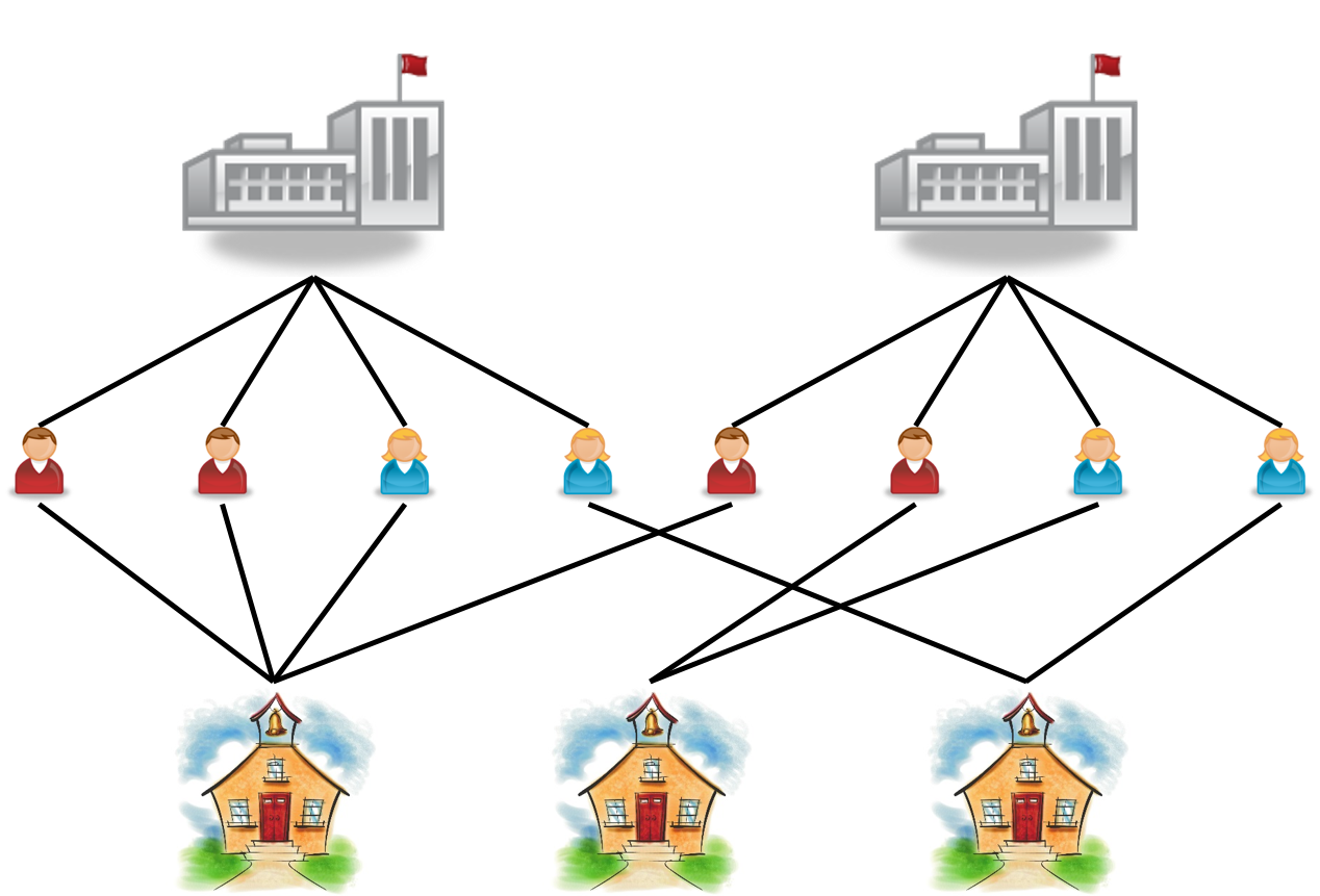
Multilevel Data Structures
- Hierarchical/Nested
- Students in schools
- Clients nested within therapists within clinics
- Employees nested within organizations
- Citizens nested within employees
- Repeated measures nested within persons

Multilevel Data Structures (Cont’d)
- Crossed
- Students cross-classified by high schools and middle schools
- Responses cross-classified by items and persons
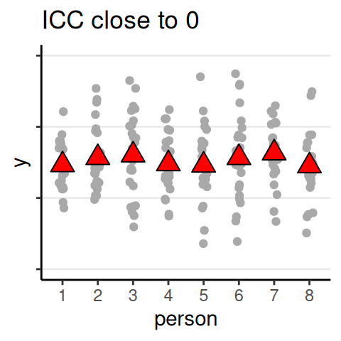
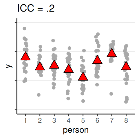
Quantifying Dependence
- Intraclass correlation (ICC): \(\rho = \dfrac{\tau^2}{\tau^2 + \sigma^2}\)
- Analogous to \(\eta^2\)/\(R^2\) effect size
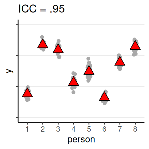
ICC
The proportion of variance of the outcome that are due to between-level (e.g., between-group, between-person) differences
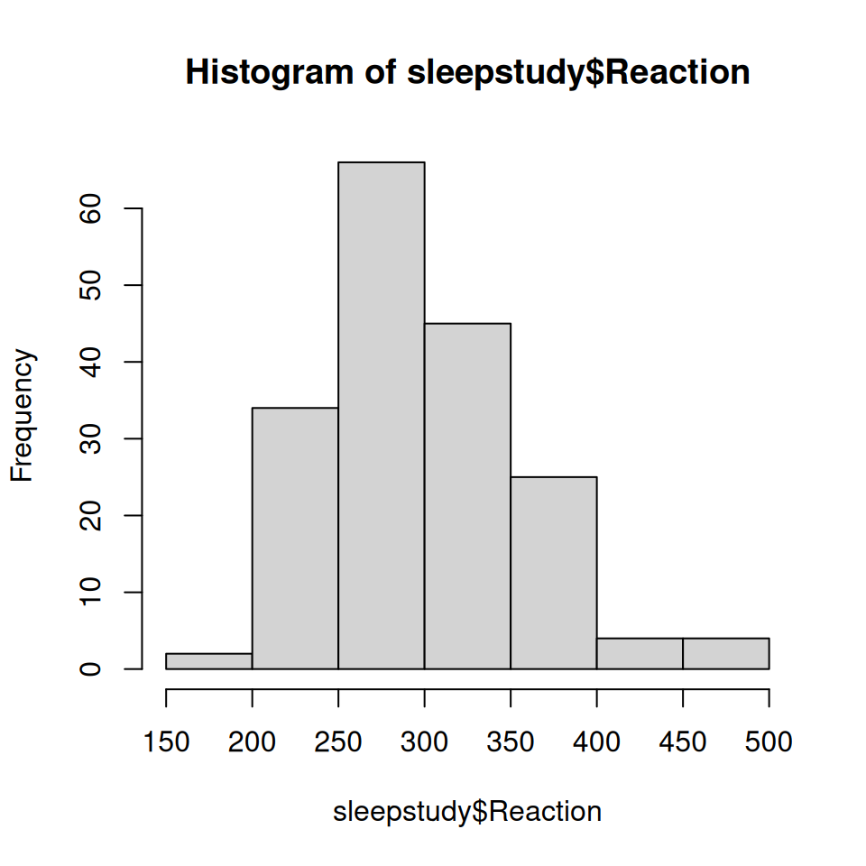
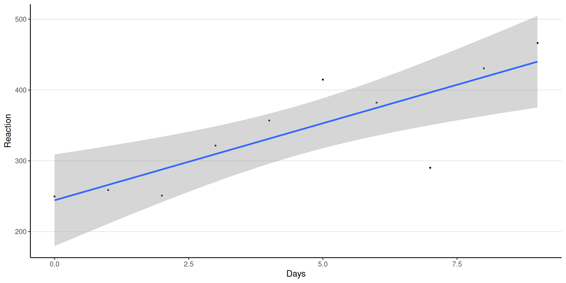
Data
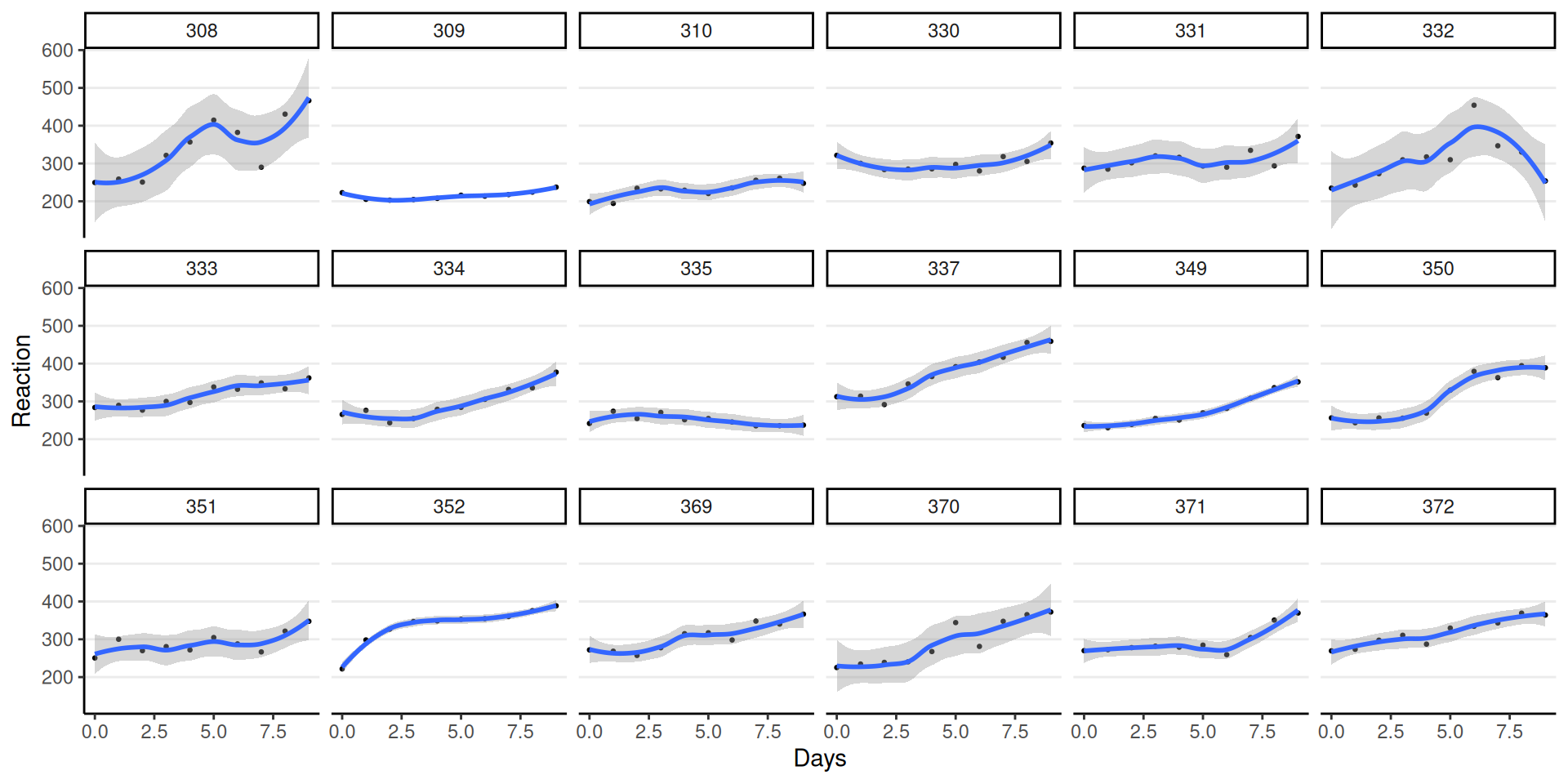
Trajectories
Interpretations
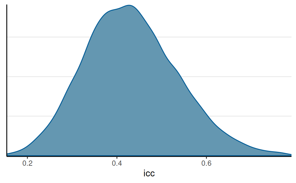
The model suggested that the average reaction time across individuals and measurement occasions was 298ms, 90% CI [281ms, 314ms]. It was estimated that 43.22%, 90% CI [27.12%, 61.31%] of the variations in reaction time was attributed to between-person differences.
Regression for One Person (308)
\[ \begin{aligned} \text{Reaction10}_i & \sim N(\mu_i, \sigma) \\ \mu_i & = \beta_0 + \beta_1 \texttt{Days}_i \end{aligned} \]
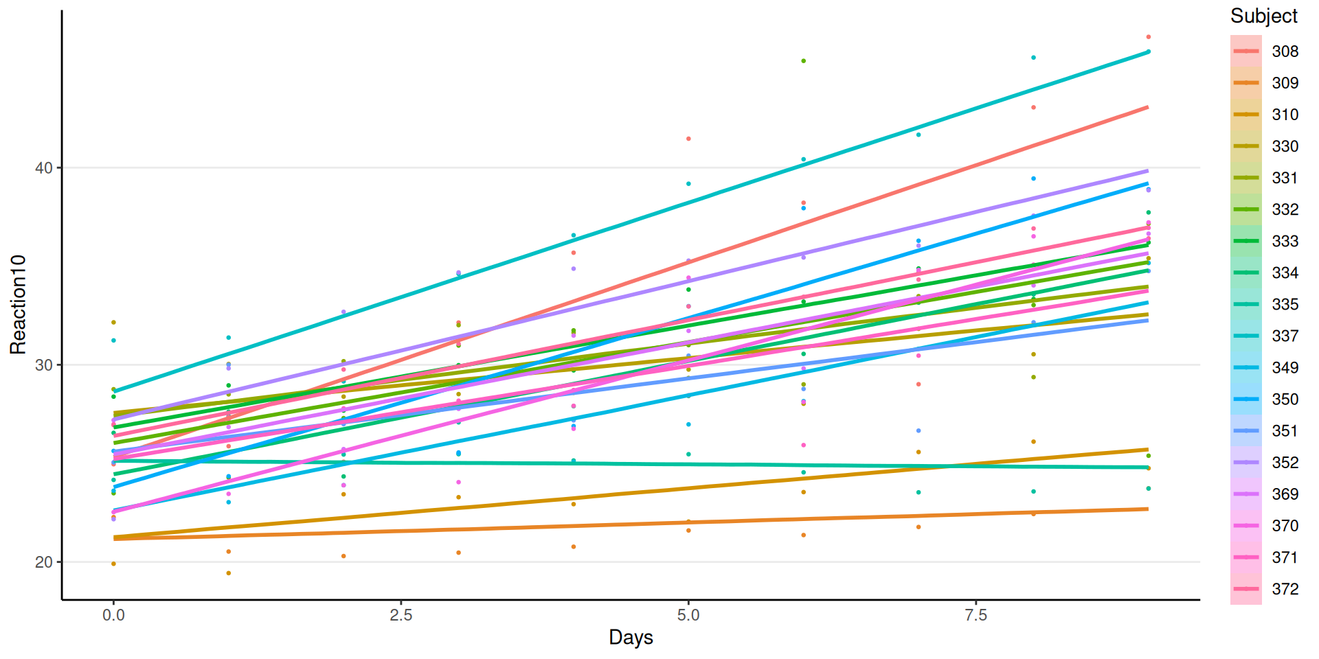
Varying Coefficients
In MLM, parameters (\(\beta_0\), \(\beta_1\), \(\sigma\)) can be
- different across clusters (persons)
- be estimated by partial pooling
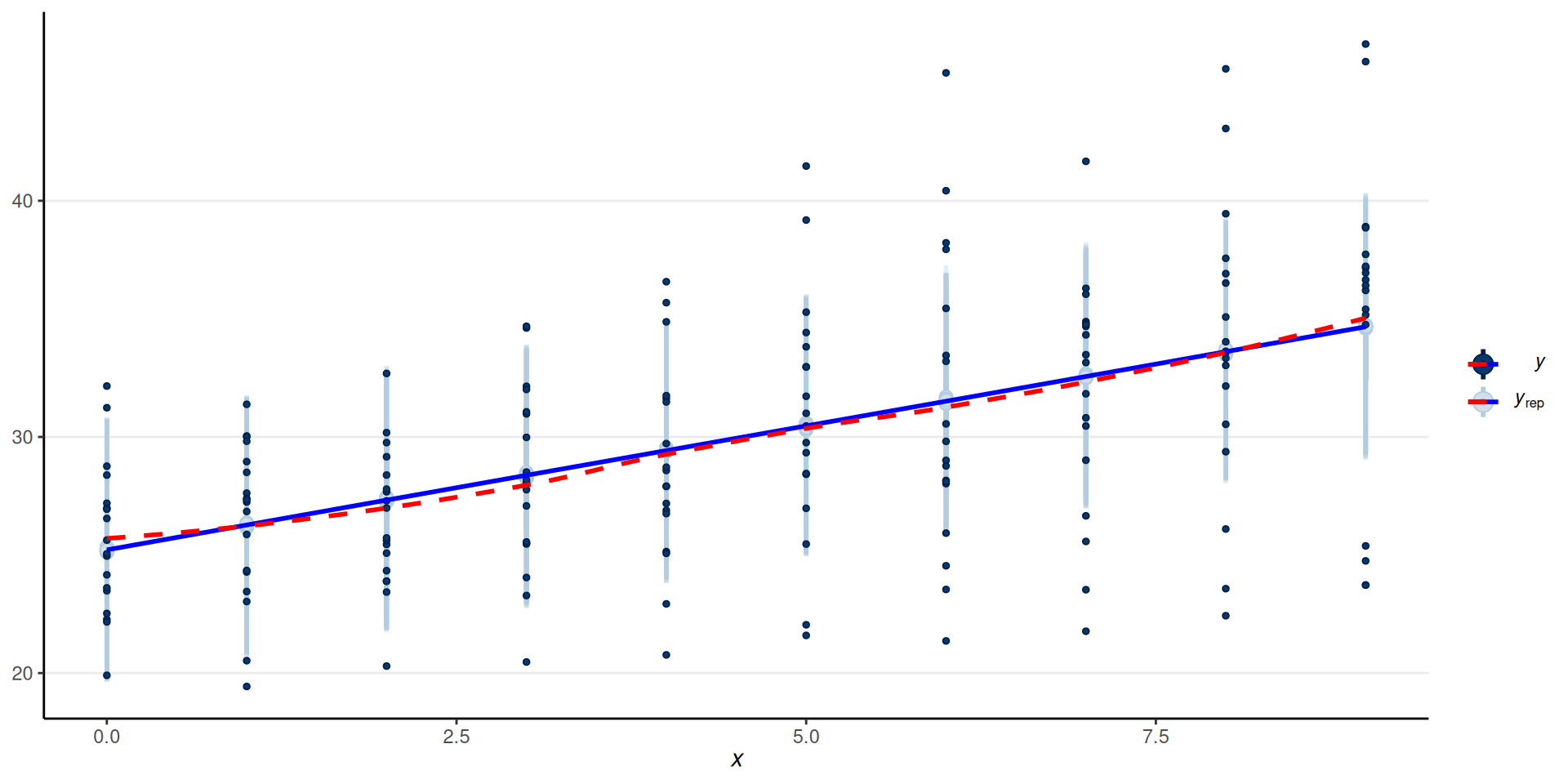
Overall Fit
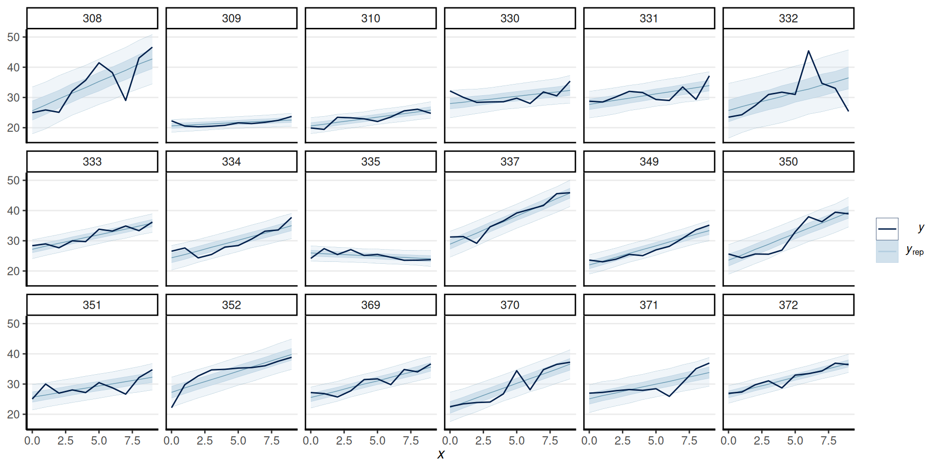
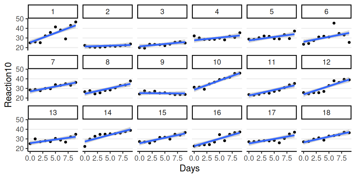
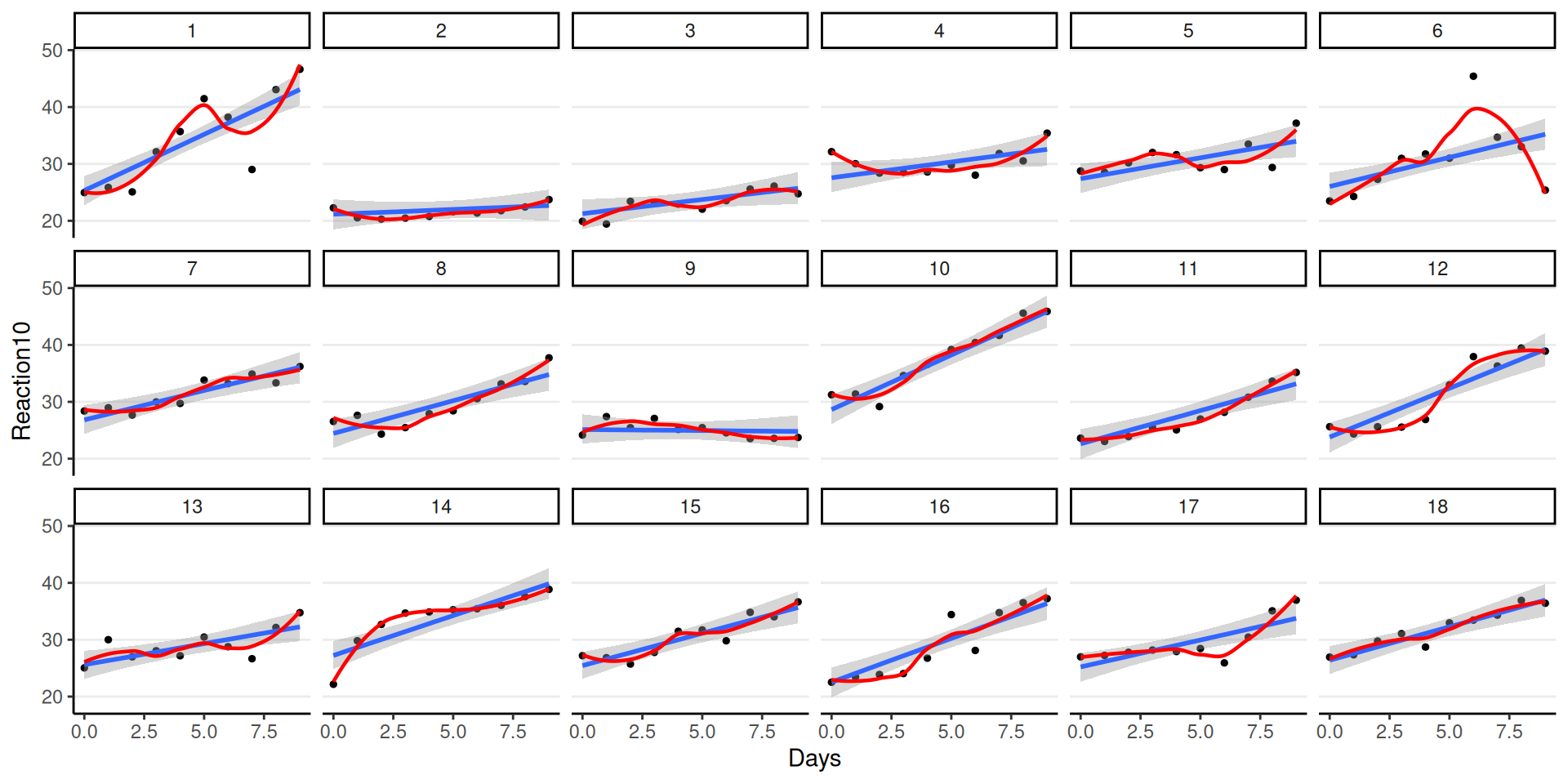
Fit to Individuals
Remember: The model assumes equal slopes for each person
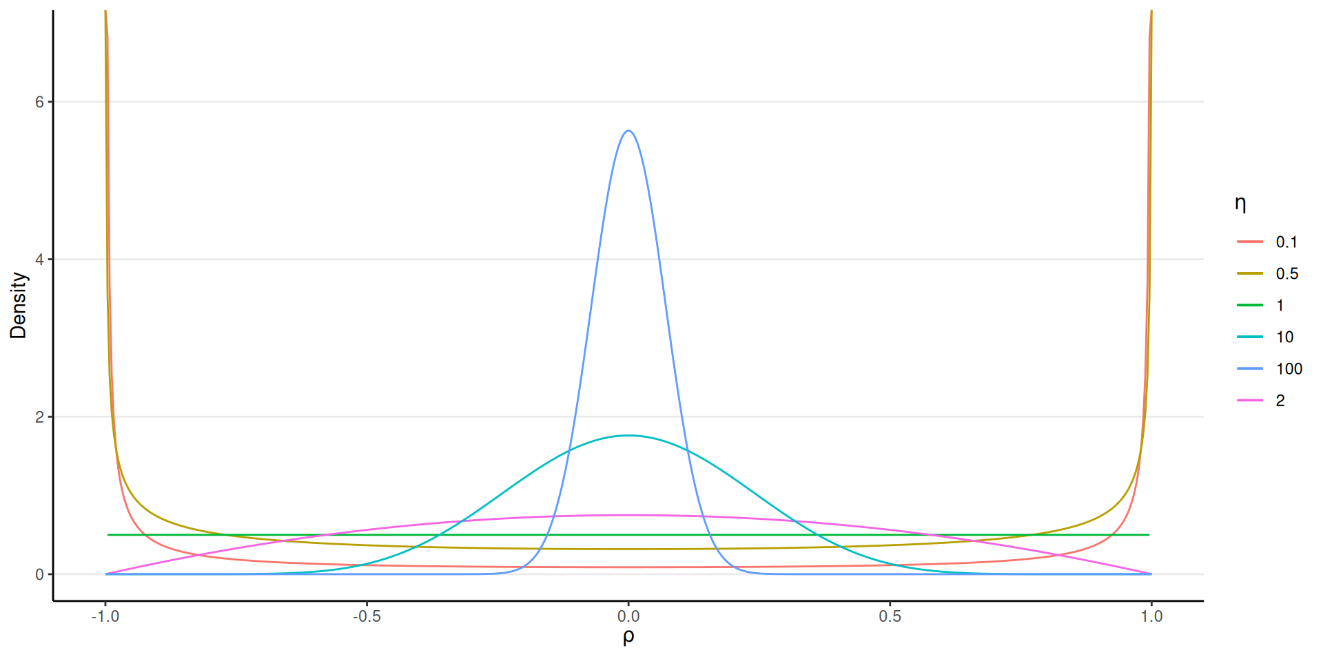
- \(\eta = 1\): Uniform
- \(\eta \geq 1\): increasingly concentrated to zero correlations
- \(\eta \leq 1\): more correlations closer to 1
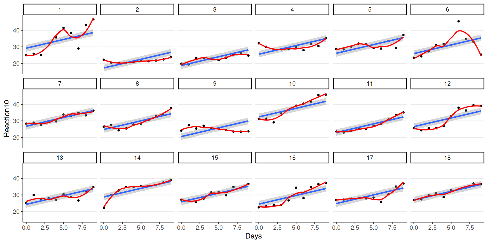
Fit to Individuals
Varying Regression Lines
Random \(\sigma\)