Model Comparison
PSYC 573
Guiding Questions
- What is overfitting and why is it problematic?
- How to measure closeness of a model to the true model?
- What do information criteria do?
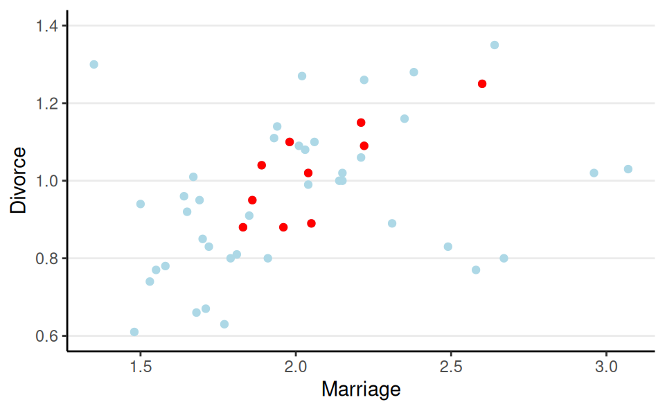
In-Sample and Out-Of-Sample Prediction
- Randomly sample 10 states
Underfitting and Overfitting
Complex models require more data
- Too few data for a complex model: overfitting
- A model being too simple: underfitting
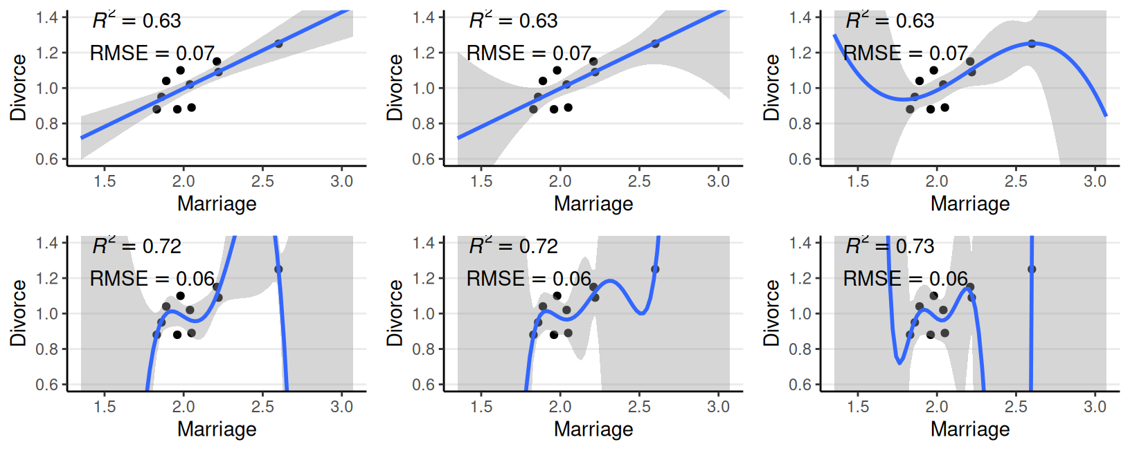
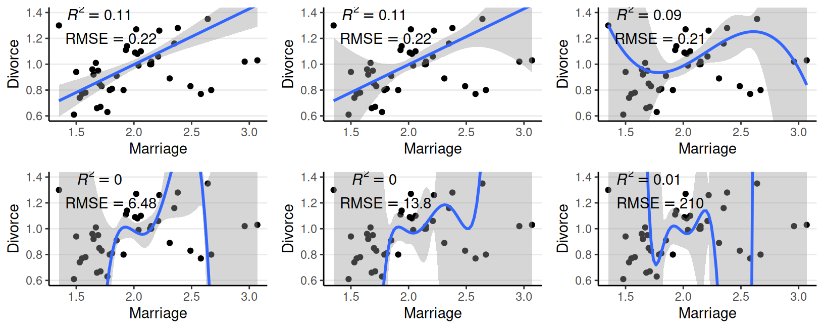
Prediction of Future Observations
- The more a model captures the noise in the original data, the less likely it predicts future observations well
Terminologies
| What it is (roughly) | Better when index is | |
|---|---|---|
| Entropy | Amount of uncertainty/information in the outcome variable(s) | — |
| KL Divergence | “Discrepancy” from “true” model | smaller |
| elpd | “Fit” to sample data | larger |
| deviance | \(-2\) \(\times\) in-sample elpd | smaller |
| AIC/WAIC | out-of-sample prediction error | smaller |
| LOOIC | out-of-sample prediction error | smaller |
What Is A Good Model?
- Closeness from the proposed model (\(M_1\)) to a “true” model (\(M_0\))
- Kullback-Leibler Divergence (\(D_\textrm{KL}\))
= \(\text{Entropy of }M_0 - \text{elpd of }M_1\) - elpd: expected log predictive density: \(E_{M_0}[\log P_{M_1}(\tilde {\mathbf{y}})]\)
- Kullback-Leibler Divergence (\(D_\textrm{KL}\))
- Choose a model with smallest \(D_\textrm{KL}\)
- When \(M_0 = M_1\), \(D_\textrm{KL} = 0\)
- \(\Rightarrow\) choose a model with largest elpd
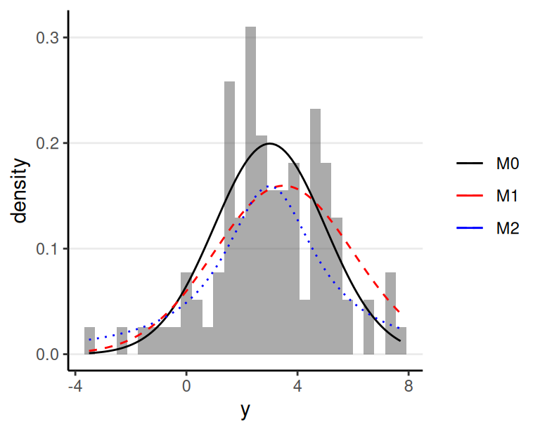
Example
- True model of data: \(M_0\): \(y \sim N(3, 2)\)
- \(M_1\): \(y \sim N(3.5, 2.5)\)
- \(M_2\): \(y \sim \mathrm{Cauchy}(3, 2)\)
Entropy of \(M_0\) = -2.112
| elpd | \(D_\textrm{KL}(M_0 \mid M_.)\) | |
|---|---|---|
| \(M_1\) | -2.175 | 0.063 |
| \(M_2\) | -2.371 | 0.259 |
Expected log pointwise predictive density
\[ \sum_i \log P_{M_1} (y_i) \]
Note: elpd is a function of sample size
- Problem: elpd depends on \(M_0\), which is unknown
- Estimate elpd using the current sample \(\rightarrow\) underestimate discrepancy
- Need to estimate elpd using an independent sample
Overfitting
Training set: 25 states; Test set: 25 remaining states
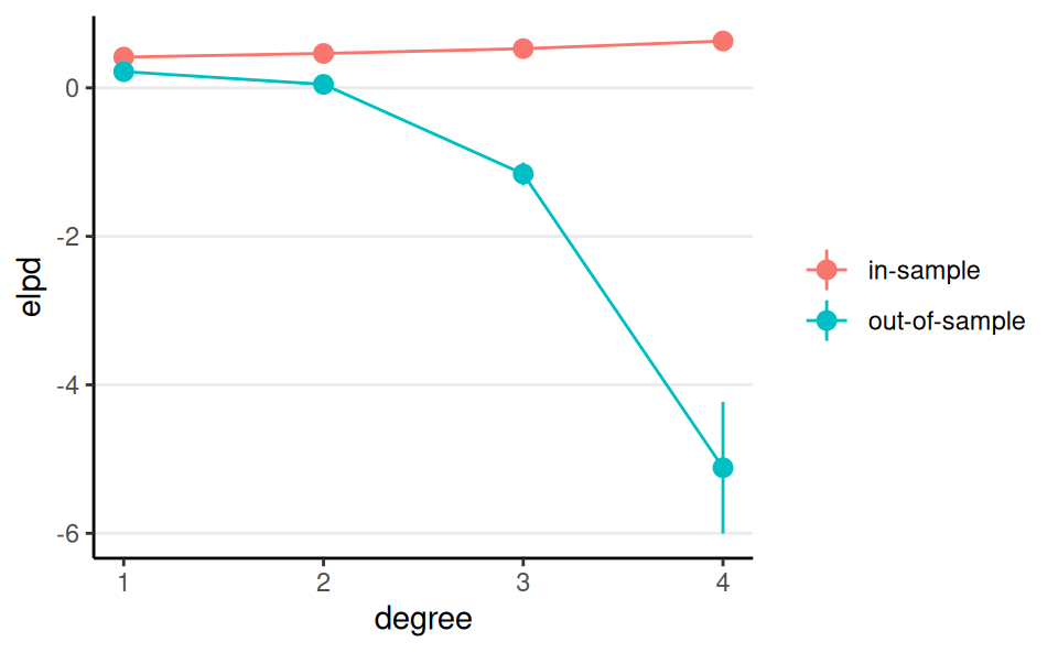
- More complex model = more discrepancy between in-sample and out-of-sample elpd
Information Criteria (IC)
Approximate discrepancy between in-sample and out-of-sample elpd
IC = \(-2\) \(\times\) (in-sample elpd \(-\) \(p\))
\(p\) = penalty for model complexity
- function of number of parameters
Choose a model with smaller IC
Bayesian ICs: DIC, WAIC, etc
Cross-Validation
Split the sample into K parts
Fit a model with K - 1 parts, and obtain elpd for the “hold-out” part
Leave-one-out: K = N
Very computationally intensive
loopackage: approximation using Pareto smoothed importance sampling
Comparing Models
\[ \texttt{Divorce}_i \sim N(\mu_i, \sigma) \]
- M1:
Marriage - M2:
Marriage,South,Marriage\(\times\)South - M3:
South, smoothing spline ofMarriagebySouth - M4:
Marriage,South,MedianAgeMarriage,Marriage\(\times\)South,Marriage\(\times\)MedianAgeMarriage,South\(\times\)MedianAgeMarriage,Marriage\(\times\)South\(\times\)MedianAgeMarriage
| M1 | M2 | M3 | M4 | |
|---|---|---|---|---|
| b_Intercept | 0.61 | 0.67 | 0.94 | 5.52 |
| b_Marriage | 0.18 | 0.13 | −1.20 | |
| b_Southsouth | −0.63 | 0.10 | 0.31 | |
| b_Marriage × Southsouth | 0.37 | 0.54 | ||
| bs_sMarriage × SouthnonMsouth_1 | −0.47 | |||
| bs_sMarriage × Southsouth_1 | 1.21 | |||
| sds_sMarriageSouthnonMsouth_1 | 0.87 | |||
| sds_sMarriageSouthsouth_1 | 0.50 | |||
| b_MedianAgeMarriage | −1.72 | |||
| b_Marriage × MedianAgeMarriage | 0.45 | |||
| b_MedianAgeMarriage × Southsouth | −0.34 | |||
| b_Marriage × MedianAgeMarriage × Southsouth | −0.09 | |||
| ELPD | 15.0 | 18.2 | 17.7 | 23.5 |
| ELPD s.e. | 5.0 | 5.5 | 5.9 | 6.2 |
| LOOIC | −30.1 | −36.5 | −35.3 | −47.1 |
| LOOIC s.e. | 9.9 | 11.0 | 11.7 | 12.3 |
| RMSE | 0.17 | 0.15 | 0.14 | 0.13 |
Notes for Using ICs
- Same outcome variable and transformation
- Same sample size
- Sample size could change when adding a predictor that has missing values
- Cannot compare discrete and continuous models
- E.g., Poisson vs. normal
Other Techniques
See notes on stacking and regularization
- Stacking: average predictions from multiple models
- Regularization: using sparsity-inducing priors to identify major predictors
- Variable selection: using projection-based methods