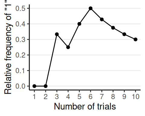
Probability and Bayes Theorem

PSYC 573

2024-09-03

History of Probability

  • Origin: To study gambling problems

  • A mathematical way to study uncertainty/randomness

Thought Experiment

Someone asks you to play a game. The person will flip a coin. You win $10 if it shows head, and lose $10 if it shows tail. Would you play?

Kolmogorov axioms

For an event \(A_i\) (e.g., getting a “1” from throwing a die)

  • \(P(A_i) \geq 0\) [All probabilities are non-negative]

  • \(P(A_1 \cup A_2 \cup \cdots) = 1\) [Union of all possibilities is 1]

  • \(P(A_1) + P(A_2) = P(A_1 \text{ or } A_2)\) for mutually exclusive \(A_1\) and \(A_2\) [Addition rule]

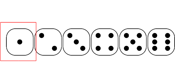
Throwing a Die With Six Faces

\(A_1\) = getting a one, . . . \(A_6\) = getting a six

  • \(P(A_i) \geq 0\)
  • \(P(\text{the number is 1, 2, 3, 4, 5, or 6}) = 1\)
  • \(P(\text{the number is 1 or 2}) = P(A_1) + P(A_2)\)

Mutually exclusive: \(A_1\) and \(A_2\) cannot both be true

Interpretations of Probability

Ways to Interpret Probability

  • Classical: Counting rules

  • Frequentist: long-run relative frequency

  • Subjectivist: Rational belief

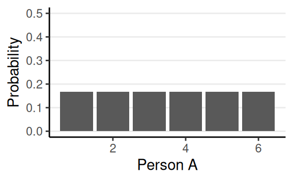
Classical Interpretation

  • Number of target outcomes / Number of possible “indifferent” outcomes
    • E.g., Probability of getting “1” when throwing a die: 1 / 6

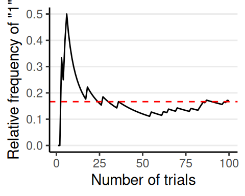
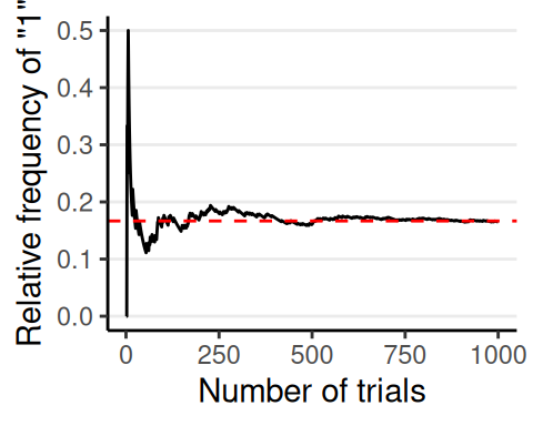
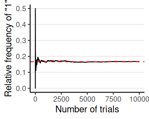
Frequentist Interpretation

  • Long-run relative frequency of an outcome
Trial Outcome
1 2
2 3
3 1
4 3
5 1
6 1
7 5
8 6
9 3
10 3

Problem of the single case

Some events cannot be repeated

  • Probability of Democrats/Republicans winning the 2024 election
  • Probability of the LA Chargers winning the 2024 Super Bowl

Or, probability that the null hypothesis is true

For frequentist, probability is not meaningful for a single case

Subjectivist Interpretation

  • State of one’s mind; the belief of all outcomes
    • Subjected to the constraints of:
      • Axioms of probability
      • That the person possessing the belief is rational

Describing a Subjective Belief

  • Assign a value for every possible outcome
    • Not an easy task
  • Use a probability distribution to approximate the belief
    • Usually by following some conventions
    • Some distributions preferred for computational efficiency

Probability Distribution

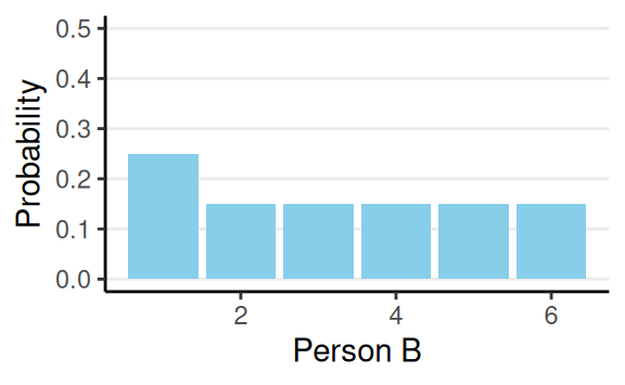
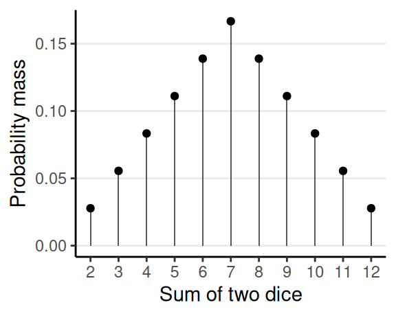
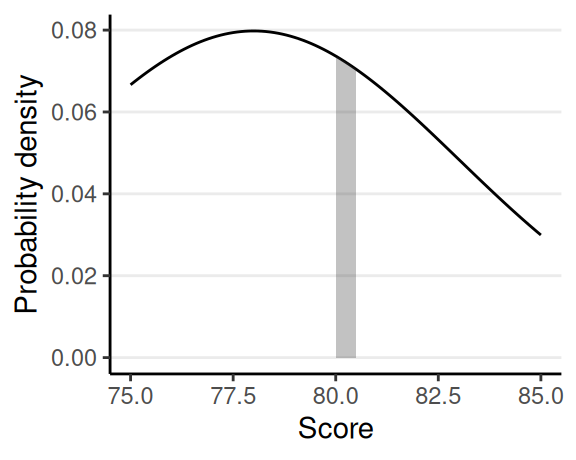
Probability Distributions

  • Discrete outcome: Probability mass

  • Continuous outcome: Probability density

Probability Density

  • If \(X\) is continuous, the probability of \(X\) having any particular value \(\to\) 0
    • E.g., probability a person’s height is 174.3689 cm

Instead, we obtain probability density: \[ P(x_0) = \lim_{\Delta x \to 0} \frac{P(x_0 < X < x_0 + \Delta x)}{\Delta x} \]

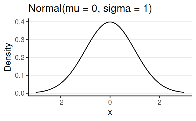
Normal Probability Density

\[ P(x) = \frac{1}{\sqrt{2 \pi} \sigma} \exp\left(-\frac{1}{2}\left[\frac{x - \mu}{\sigma}\right]^2\right) \]

my_normal_density <- function(x, mu, sigma) {
    exp(- ((x - mu) / sigma) ^2 / 2) / (sigma * sqrt(2 * pi))
}

Some Commonly Used Distributions

Summarizing a Probability Distribution

Central tendency

The center is usually the region of values with high plausibility

  • Mean, median, mode

Dispersion

How concentrated the region with high plausibility is

  • Variance, standard deviation
  • Median absolute deviation (MAD)

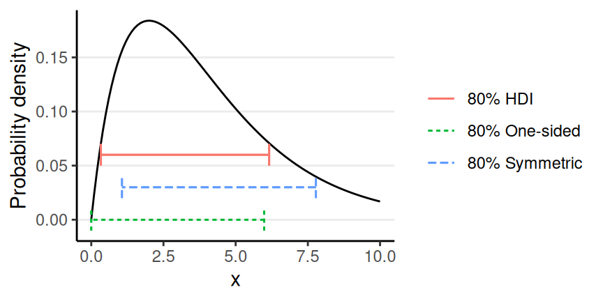
Summarizing a Probability Distribution (cont’d)

Interval

  • One-sided
  • Symmetric
  • Highest density interval (HDI)

Multiple Variables

  • Joint probability: \(P(X, Y)\)
  • Marginal probability: \(P(X)\), \(P(Y)\)

>= 4 <= 3 Marginal (odd/even)
odd 1/6 2/6 3/6
even 2/6 1/6 3/6
Marginal (>= 4 or <= 3) 3/6 3/6 1

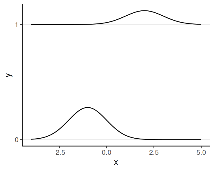
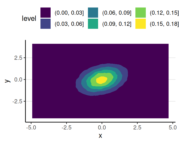
Multiple Continuous Variables

  • Left: Continuous \(X\), Discrete \(Y\)
  • Right: Continuous \(X\) and \(Y\)

Conditional Probability

Knowing the value of \(B\), the relative plausibility of each value of outcome \(A\)

\[ P(A \mid B_1) = \frac{P(A, B_1)}{P(B_1)} \]

E.g., P(Alzheimer’s) vs. P(Alzheimer’s | family history)

E.g., Knowing that the number is odd

>= 4 <= 3
odd 1/6 2/6
even 2/6 1/6
Marginal (>= 4 or <= 3) 3/6 3/6

Conditional = Joint / Marginal

>= 4 <= 3
odd 1/6 2/6
Marginal (>= 4 or <= 3) 3/6 3/6
Conditional (odd) (1/6) / (3/6) = 1/3 (1/6) / (2/6) = 2/3

\(P(A \mid B) \neq P(B \mid A)\)

  • \(P\)(number is six | even number) = 1 / 3

  • \(P\)(even number | number is six) = 1

Another example:

\(P\)(road is wet | it rains) vs. \(P\)(it rains | road is wet)

  • Problem: Not considering other conditions leading to wet road: sprinkler, street cleaning, etc

Sometimes called the confusion of the inverse

Independence

\(A\) and \(B\) are independent if

\[ P(A \mid B) = P(A) \]

E.g.,

  • \(A\): A die shows five or more
  • \(B\): A die shows an odd number

P(>= 5) = 1/3. P(>=5 | odd number) = ? P(>=5 | even number) = ?

P(<= 5) = 2/3. P(<=5 | odd number) = ? P(>=5 | even number) = ?

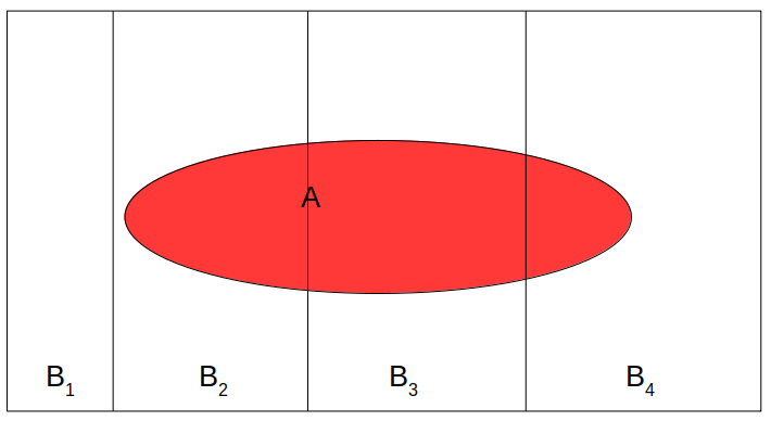
Law of Total Probability

From conditional \(P(A \mid B)\) to marginal \(P(A)\)

  • If \(B_1, B_2, \cdots, B_n\) are all possibilities for an event (so they add up to a probability of 1), then

\[ \begin{align} P(A) & = P(A, B_1) + P(A, B_2) + \cdots + P(A, B_n) \\ & = P(A \mid B_1)P(B_1) + P(A \mid B_2)P(B_2) + \cdots + P(A \mid B_n) P(B_n) \\ & = \sum_{k = 1}^n P(A \mid B_k) P(B_k) \end{align} \]
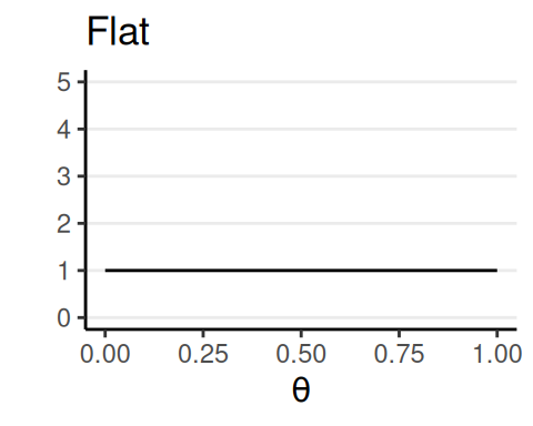
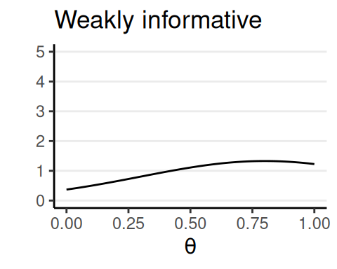
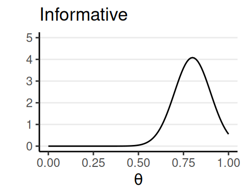
Example

Consider the use of a depression screening test for people with diabetes. For a person with depression, there is an 85% chance the test is positive. For a person without depression, there is a 28.4% chance the test is positive. Assume that 19.1% of people with diabetes have depression. If the test is given to 1,000 people with diabetes, around how many people will be tested positive?

Bayes Theorem

Bayes Theorem

Given \(P(A, B) = P(A \mid B) P(B) = P(B \mid A) P(A)\) (joint = conditional \(\times\) marginal)

\[ P(B \mid A) = \dfrac{P(A \mid B) P(B)}{P(A)} \]

Which says how we can go from \(P(A \mid B)\) to \(P(B \mid A)\)

Consider \(B_i\) \((i = 1, \ldots, n)\) as one of the many possible mutually exclusive events

\[ \begin{aligned} P(B_i \mid A) & = \frac{P(A \mid B_i) P(B_i)}{P(A)} \\ & = \frac{P(A \mid B_i) P(B_i)}{\sum_{k = 1}^n P(A \mid B_k)P(B_k)} \end{aligned} \]

Example

A police officer stops a driver at random and does a breathalyzer test for the driver. The breathalyzer is known to detect true drunkenness 100% of the time, but in 1% of the cases, it gives a false positive when the driver is sober. We also know that in general, for every 1,000 drivers passing through that spot, one is driving drunk. Suppose that the breathalyzer shows positive for the driver. What is the probability that the driver is truly drunk?

Bayesian Data Analysis

Bayes Theorem in Data Analysis

  • Bayesian statistics
    • more than applying Bayes theorem
    • a way to quantify the plausibility of every possible value of some parameter \(\theta\)
      • E.g., population mean, regression coefficient, etc
    • Goal: update one’s Belief about \(\theta\) based on the observed data \(D\)

Going back to the example

Goal: Find the probability that the person is drunk, given the test result

Parameter (\(\theta\)): drunk (values: drunk, sober)

Data (\(D\)): test (possible values: positive, negative)

Bayes theorem: \(\underbrace{P(\theta \mid D)}_{\text{posterior}} = \underbrace{P(D \mid \theta)}_{\text{likelihood}} \underbrace{P(\theta)}_{\text{prior}} / \underbrace{P(D)}_{\text{marginal}}\)

Usually, the marginal is not given, so

\[ P(\theta \mid D) = \frac{P(D \mid \theta)P(\theta)}{\sum_{\theta^*} P(D \mid \theta^*)P(\theta^*)} \]

  • \(P(D)\) is also called evidence, or the prior predictive distribution
    • E.g., probability of a positive test, regardless of the drunk status

Example 2

shiny::runGitHub("plane_search", "marklhc")
  • Try choosing different priors. How does your choice affect the posterior?
  • Try adding more data. How does the number of data points affect the posterior?

The posterior is a synthesis of two sources of information: prior and data (likelihood)

Generally speaking, a narrower distribution (i.e., smaller variance) means more/stronger information

  • Prior: narrower = more informative/strong
  • Likelihood: narrower = more data/more informative

Priors

Prior beliefs used in data analysis must be admissible by a skeptical scientific audience (Kruschke, 2015, p. 115)

  • Flat, noninformative, vague
  • Weakly informative: common sense, logic
  • Informative: publicly agreed facts or theories

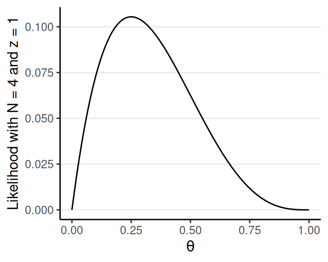
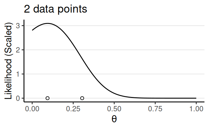
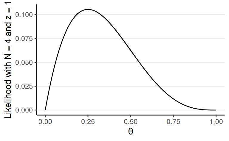
Likelihood/Model/Data \(P(D \mid \theta, M)\)

Probability of observing the data as a function of the parameter(s)

  • Also written as \(L(\theta \mid D)\) or \(L(\theta; D)\) to emphasize it is a function of \(\theta\)
  • Also depends on a chosen model \(M\): \(P(D \mid \theta, M)\)

Likelihood of Multiple Data Points

  1. Given \(D_1\), obtain posterior \(P(\theta \mid D_1)\)
  2. Use \(P(\theta \mid D_1)\) as prior, given \(D_2\), obtain posterior \(P(\theta \mid D_1, D_2)\)

The posterior is the same as getting \(D_2\) first then \(D_1\), or \(D_1\) and \(D_2\) together, if

  • data-order invariance is satisfied, which means
  • \(D_1\) and \(D_2\) are exchangeable

Exchangeability

Joint distribution of the data does not depend on the order of the data

E.g., \(P(D_1, D_2, D_3) = P(D_2, D_3, D_1) = P(D_3, D_2, D_1)\)

Example of non-exchangeable data:

  • First child = male, second = female vs. first = female, second = male
  • \(D_1, D_2\) from School 1; \(D_3, D_4\) from School 2 vs. \(D_1, D_3\) from School 1; \(D_2, D_4\) from School 2

Bernoulli Example

Coin Flipping: Binary Outcomes

Q: Estimate the probability that a coin gives a head

  • \(\theta\): parameter, probability of a head

Flip a coin, showing head

  • \(y = 1\) for showing head

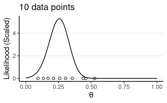
Multiple Binary Outcomes

Bernoulli model is natural for binary outcomes

Assume the flips are exchangeable given \(\theta\), \[ \begin{align} P(y_1, \ldots, y_N \mid \theta) &= \prod_{i = 1}^N P(y_i \mid \theta) \\ &= \theta^z (1 - \theta)^{N - z} \end{align} \]

\(z\) = # of heads; \(N\) = # of flips
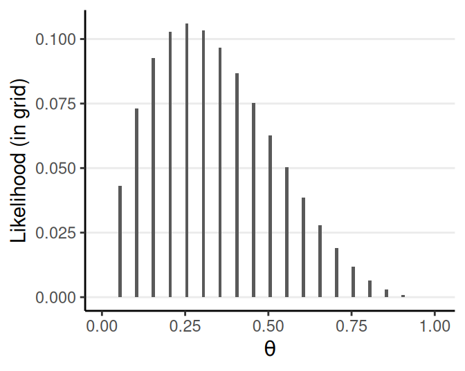
Posterior

Same posterior, two ways to think about it

Prior belief, weighted by the likelihood

\[ P(\theta \mid y) \propto \underbrace{P(y \mid \theta)}_{\text{weights}} P(\theta) \]

Likelihood, weighted by the strength of prior belief

\[ P(\theta \mid y) \propto \underbrace{P(\theta)}_{\text{weights}} P(\theta \mid y) \]

Grid Approximation

See Exercise 2

Discretize a continuous parameter into a finite number of discrete values

For example, with \(\theta\): [0, 1] \(\to\) [.05, .15, .25, …, .95]

Criticism of Bayesian Methods

Criticism of “Subjectivity”

Main controversy: subjectivity in choosing a prior

  • Two people with the same data can get different results because of different chosen priors

Counters to the Subjectivity Criticism

  • With enough data, different priors hardly make a difference
  • Prior: just a way to express the degree of ignorance
    • One can choose a weakly informative prior so that the Influence of subjective Belief is small

Counters to the Subjectivity Criticism 2

Subjectivity in choosing a prior is

  • Same as in choosing a model, which is also done in frequentist statistics
  • Relatively strong prior needs to be justified,
    • Open to critique from other researchers
  • Inter-subjectivity \(\rightarrow\) Objectivity

Counters to the Subjectivity Criticism 3

The prior is a way to incorporate previous research efforts to accumulate scientific evidence

Why should we ignore all previous literature every time we conduct a new study?