One Parameter Models

PSYC 573

2024-09-10

Bernoulli Model

Data (Subsample)

Patients diagnosed with AIDS in Australia before 1 July 1991

state	sex	diag	death	status	T.categ	age
VIC	M	1991-03-05	1991-07-01	A	hs	36
NSW	M	1987-08-30	1988-03-11	D	hs	25
QLD	M	1989-10-09	1990-08-22	D	hs	36
NSW	M	1991-03-17	1991-07-01	A	hs	42
NSW	M	1986-04-12	1989-01-31	D	hs	40
NSW	M	1986-09-29	1987-03-25	D	hs	69
NSW	M	1989-08-24	1991-07-01	A	hs	37
Other	F	1988-10-19	1991-07-01	A	id	30
NSW	M	1990-04-07	1991-01-21	D	hs	30
NSW	M	1988-04-28	1990-04-07	D	hs	41

Cpc chine at English Wikipedia, CC BY-SA 3.0 https://creativecommons.org/licenses/by-sa/3.0, via Wikimedia Commons

Let’s go through the Bayesian workflow

flowchart LR
  subgraph DATA
    direction TB
    A[Identify/Collect Data] --> B[Visualize Data]
  end
    %% B --> C[Choose/Modify Model]
  subgraph MODEL
    H -->|Model fit not satisfactory|C
    C[Choose/Modify Model] --> D[Specify Priors]
    D --> E[Prior Predictive Check]
    E --> G[MCMC Sampling with Convergence diagnostics]
    G --> H[Posterior Predictive Check]
  end
  subgraph RESULTS
    %% I -->|Model is reasonable|J[Model comparisons/averaging]
    J[Model comparisons/averaging] --> K[Interpret and Visualize Results]
  end
  DATA --> MODEL
  MODEL --> RESULTS

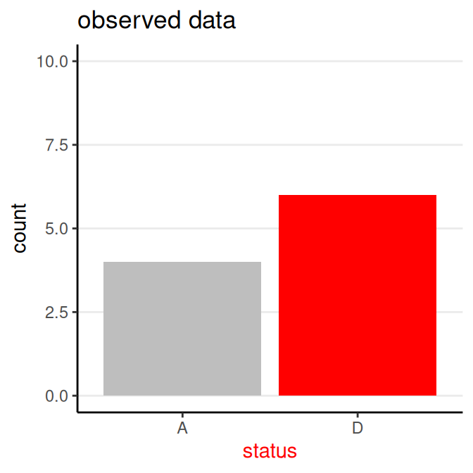
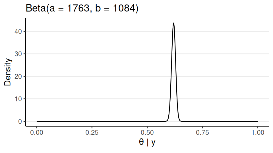
Choose a Model: Bernoulli

Data: \(y\) = survival status (0 = “A”, 1 = “D”)

Parameter: \(\theta\) = probability of “D”

Model equation: \(y_i \sim \text{Bern}(\theta)\) for \(i = 1, 2, \ldots, N\)

The model states:

the sample data \(y\) follows a Bernoulli distribution with the common parameter \(\theta\)

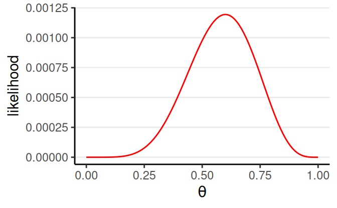
Bernoulli Likelihood

Notice that there is no subscript for \(\theta\):

The model assumes each observation has the same \(\theta\)
I.e., the observations are exchangeable

\[ P(y_1, y_2, \ldots, y_N) = \theta^z (1 - \theta)^{N - z} \]

\(z\) = number of “successes” (“D”)

\(z\) = 6 in this illustrative sample

theta	likelihood
0.0	0.00000
0.1	0.00000
0.2	0.00003
0.3	0.00018
0.4	0.00053
0.5	0.00098
0.6	0.00119
0.7	0.00095
0.8	0.00042
0.9	0.00005
1.0	0.00000

Choosing Priors

When choosing priors, start with the support of the parameter(s)

Support: Values that are possible

Support for \(\theta\): [0, 1]

One possible (but unlikely) option

\(\theta\) values in the range \([.40, .60)\) are 5 times more likely than any values outside of that range

Conjugate Prior: Beta Distribution

\[ P(\theta \mid a, b) \propto \theta^{a - 1} (1 - \theta)^{b - 1} I_{[0, 1]} \]

a <- 1
b <- 1
dbeta(theta1, shape1 = a, shape2 = b)

Conjugate Prior

A prior distribution that yields posterior in the same distribution family as the prior

Two hyperparameters, \(a\) and \(b\):

\(a - 1\) = number of prior ‘successes’ (e.g., “D”)
\(b - 1\) = number of prior ‘failures’

Obtaining the Posterior Analytically

\[ P(\theta \mid y) = \frac{P(y \mid \theta) P(\theta)}{\int_0^1 P(y \mid \theta^*) P(\theta^*) d \theta^*} \]

The denominator is usually intractable

Conjugate prior: Posterior is from a known distribution family

\(N\) trials and \(z\) successes
\(\mathrm{Beta}(a, b)\) prior
\(\Rightarrow\) \(\mathrm{Beta}(a + z, b + N - z)\) posterior
- \(a + \color{red}{z} - 1\) successes
- \(b + \color{red}{N - z} - 1\) failures

Back to the Example

\(N\) = 10, \(z\) = 6

Prior: Do you believe that the fatality rate of AIDS is 100%? or 0%?

Let’s use \(\kappa = 4\), prior mean = 0.5, so \(a\) = 2 and \(b\) = 2

Posterior Beta

\[ \theta \mid y \sim \mathrm{Beta}(2 + 6, 2 + 4) \]

ggplot(data.frame(x = c(0, 1)), aes(x = x)) +
    stat_function(fun = dbeta,
                  args = list(shape1 = 8, shape2 = 6)) +
    labs(title = "Beta(a = 8, b = 6)",
         x = expression(theta), y = "Density")

Summarizing the Posterior

If the posterior is from a known family, one can evalue summary statistics analytically

E.g., \(E(\theta \mid y) = \int_0^1 \theta P(\theta \mid y) d \theta\)

However, more often, a simulation-based approach is used to draw samples from the posterior

num_draws <- 1000
sim_theta <- rbeta(1000, shape1 = 8, shape2 = 6)

Statistic	Common Name	Value
mean	Bayes estimate/Expected a posteriori (EAP)	0.563
median	Posterior median	0.567
mode	Maximum a posteriori (MAP)	0.577
SD	Posterior SD	0.126
MAD	Posterior MAD	0.13
80% CI	(Equal-tailed) Credible interval	[0.398, 0.727]
80% HDI	HDI/Highest Posterior Density Interval (HPDI)	[0.404, 0.733]

Using the Full Data

1082 A, 1761 D \(\rightarrow\) \(N\) = 2843, \(z\) = 1761

Posterior: Beta(1763, 1084)

Posterior Predictive Check

Posterior Predictive Distribution

\[ P(\tilde y \mid y) = \int P(\tilde y \mid \theta, y) P(\theta \mid y) d \theta \]

\(\tilde y\) = new/future data

Simulate a new \(\theta^*\) from posterior, then simulate a new data set

If the model does not fit the data, any results are basically meaningless at best, and can be very misleading

Requires substantive knowledge and some creativity

E.g., are the case fatality rates equal across the 4 state categories?

1theta_new <- rbeta(1, 1763, 1084)
2status_new <- sample(c("D", "A"), nrow(Aids2),
    replace = TRUE, prob = c(theta_new, 1 - theta_new)
)
df_new <- Aids2 |>
    mutate(status = factor(status_new))

1: Sample a new theta from the posterior
2: Sample new data based on the new theta

Some Common Checks

Does the model simulate data with similar distributions as the observed data?
- e.g., skewness, range
Subsets of observed data that are of more interest?
- e.g., old age group
- If not fit, age should be incorporated in the model

See an example in Gabry et al. (2019)

Stan

See notes

Stan Example

data {
  int<lower=0> N;  // number of observations
  array[N] int<lower=0,upper=1> y;  // y
}
parameters {
  real<lower=0,upper=1> theta;  // theta parameter
}
model {
  theta ~ beta(2,2);  // prior: Beta(2, 2)
  y ~ bernoulli(theta);  // model: Bernoulli
}

bern_mod <- cmdstan_model("stan_code/beta-bernoulli.stan")
fit <- bern_mod$sample(Aids2_standata)

Example Check: Sample mean by age group

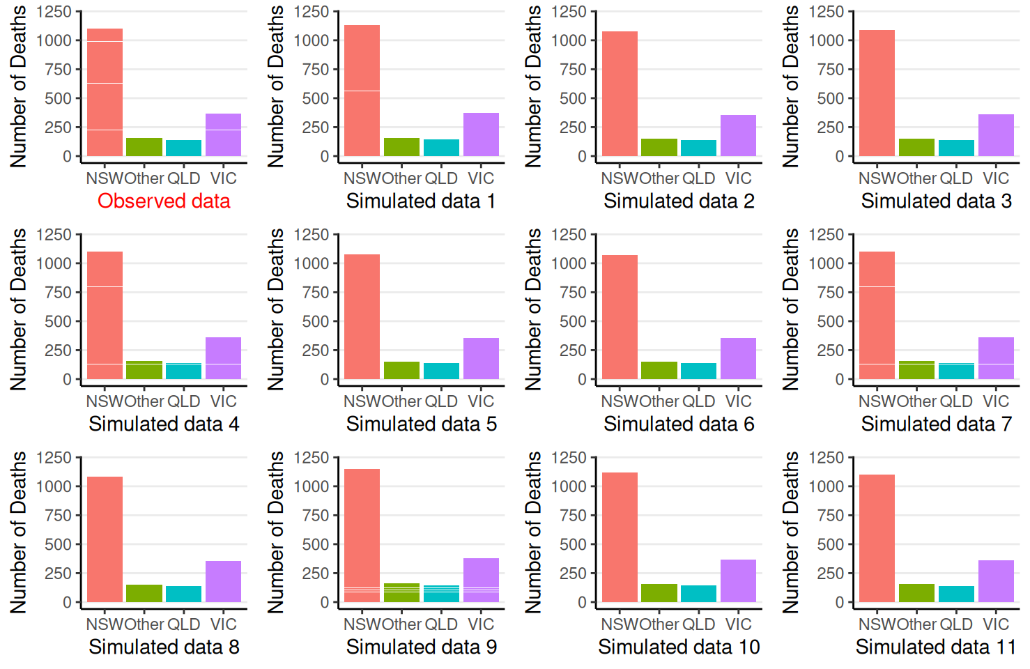
Here we use the function bayesplot::ppc_stat_grouped()

1age50 <- factor(Aids2$age > 50, labels = c("<= 50", "> 50"))
2bern_pp_fit$draws("ytilde", format = "draws_matrix") |>
3    ppc_stat_grouped(y = Aids2_standata$y, group = age50, stat = "mean")

1: Create binary indicator of two age groups
2: Extract simulated data sets
3: Plot a histogram of the sample means from the simulated data (i.e., posterior predictive distribution) for each age group

Other One-Parameter Models

Binomial Model

For count outcome: \(y_i \sim \mathrm{Bin}(N_i, \theta)\)
- \(\theta\): rate of occurrence (per trial)
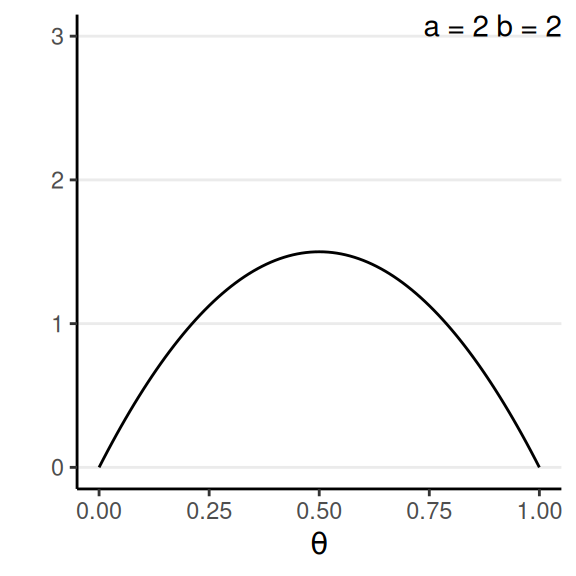
Conjugate prior: Beta
E.g.,
- \(y\) minority candidates in \(N\) new hires
- \(y\) out of \(N\) symptoms checked
- A word appears \(y\) times in a tweet of \(N\) number of words

Poisson Model

For count outcome: \(y_i \sim \mathrm{Pois}(\theta)\)
- \(\theta\): rate of occurrence
Conjugate prior: Gamma
E.g.,
- Drinking \(y\) times in a week
- \(y\) hate crimes in a year for a county
- \(y\) people visiting a store in an hour

Bibliography

Gabry, Jonah, Daniel Simpson, Aki Vehtari, Michael Betancourt, and Andrew Gelman. 2019. “Visualization in Bayesian Workflow.” Journal of the Royal Statistical Society Series A: Statistics in Society 182 (2): 389–402. https://doi.org/10.1111/rssa.12378.

Gelman, Andrew, Aki Vehtari, Daniel Simpson, Charles C. Margossian, Bob Carpenter, Yuling Yao, Lauren Kennedy, Jonah Gabry, Paul-Christian Bürkner, and Martin Modrák. 2020. “Bayesian Workflow.” arXiv. https://doi.org/10.48550/ARXIV.2011.01808.

One Parameter Models

Bernoulli Model

Data (Subsample)

Choose a Model: Bernoulli

Bernoulli Likelihood

Choosing Priors

Conjugate Prior: Beta Distribution

More on the Beta Distribution

Obtaining the Posterior Analytically

Back to the Example

Posterior Beta

Summarizing the Posterior

Using the Full Data

Posterior Predictive Check

Some Common Checks

Stan

Stan Example

Example Check: Sample mean by age group

Other One-Parameter Models

Binomial Model

Poisson Model

Bibliography