5 Beta-Bernoulli Model With Stan
In the previous lecture, we fitted a Beta-Bernoulli model using Gibbs sampling with our own R code. While this is doable in this relatively simple model (it only has one parameter), for more complex models, Gibbs sampling and other MCMC methods (to be introduced in a later class) require quite a lot of programming. Fortunately for us, we have some readily available software for doing MCMC. While it is probably overkill for the Beta-Bernoulli model, we will learn working with Stan by using it to analyze the Beta-Bernoulli model. Specifically, we will learn to:
- Install Stan and the R package
cmdstanrfor communicating between R and Stan; - Write Stan code for the Beta-Bernoulli model;
- Draw posterior samples using Stan;
- Summarize and plot the posterior samples.
We will talk about convergence of MCMC, which is an extremely important topic, in a later class.
5.1 Installing Stan
- Follow the steps in https://mc-stan.org/cmdstanr/ to install the
cmdstanrpackage. - Load the
cmdstanrpackage, and runinstall_cmdstan()
- If you run into an error in the previous step related to C++ toolchain, follow the directions here: https://mc-stan.org/cmdstanr/articles/cmdstanr.html
5.2 Fitting a Beta-Bernoulli Model in Stan
5.2.1 Data Import
From last class:
5.2.2 Writing Stan syntax
Stan has its own syntax and is different from R. For example, we want to fit the following Beta-Bernoulli model:
\[ \begin{aligned} y_i & \sim \text{Bern}(\theta) \text{ for }i = 1, 2, \ldots, N \\ P(\theta) & \sim \text{Beta}(2, 2) \end{aligned} \]
and the model can be written in Stan as follows:
data {
  int<lower=0> N;  // number of observations
  array[N] int<lower=0,upper=1> y;  // y
}
parameters {
  real<lower=0,upper=1> theta;  // theta parameter
}
model {
  theta ~ beta(2,2);  // prior: Beta(2, 2)
  y ~ bernoulli(theta);  // model: Bernoulli
}
Save the above model syntax in a separate file ending in .stan. For example, I saved the syntax in the file beta-bernoulli.stan in a folder named stan_code.
In Stan, anything after // denotes comments (like # in R) and will be ignored by the program. In each block (e.g., data {}), a statement should end with a semicolon (;). There are several blocks in the above Stan code:
-
data: The data input for Stan is usually not only an R data frame, but a list that includes other information, such as sample size, number of predictors, and prior scales. Each type of data has an input type, such asint= integer,real= numbers with decimal places,matrix= 2-dimensional data of real numbers,vector= 1-dimensional data of real numbers, andarray= 1- to many-dimensional data. For example, we usearray[N]for the data type ofy, because it is a vector, but each element is an integer (and cannot take decimals).
We can set the lower and upper bounds so that Stan can check the input data. In the above, we used
<lower=0,upper=1>. parameters: The parameters to be estimatedtransformed parameters: optional variables that are transformations of the model parameters. It is usually used for more advanced models to allow more efficient MCMC sampling.model: It includes expressions of prior distributions for each parameter and the likelihood for the data. There are many possible distributions that can be used in Stan.generated quantities: Any quantities that are not part of the model but can be computed from the parameters for every iteration. Examples include posterior generated samples, effect sizes, and log-likelihood (for fit computation). We will see an example later.
5.2.3 Compiling the Stan model from R
To compile the model, we can call the cmdstan_model function in cmdstanr:
bern_mod <- cmdstan_model("stan_code/beta-bernoulli.stan")5.2.4 Posterior Sampling
We need to first prepare the data for input to Stan. In the Stan code, we have two objects in the data block: N and y, so we need to have a list of two elements in R:
Aids2_standata <- list(
    N = nrow(Aids2),
    y = as.integer(Aids2$status == "D")  # integer
)
Now we can draw posterior samples:
fit <- bern_mod$sample(Aids2_standata)Running MCMC with 4 sequential chains...
Chain 1 Iteration: 1 / 2000 [ 0%] (Warmup)
Chain 1 Iteration: 100 / 2000 [ 5%] (Warmup)
Chain 1 Iteration: 200 / 2000 [ 10%] (Warmup)
Chain 1 Iteration: 300 / 2000 [ 15%] (Warmup)
Chain 1 Iteration: 400 / 2000 [ 20%] (Warmup)
Chain 1 Iteration: 500 / 2000 [ 25%] (Warmup)
Chain 1 Iteration: 600 / 2000 [ 30%] (Warmup)
Chain 1 Iteration: 700 / 2000 [ 35%] (Warmup)
Chain 1 Iteration: 800 / 2000 [ 40%] (Warmup)
Chain 1 Iteration: 900 / 2000 [ 45%] (Warmup)
Chain 1 Iteration: 1000 / 2000 [ 50%] (Warmup)
Chain 1 Iteration: 1001 / 2000 [ 50%] (Sampling)
Chain 1 Iteration: 1100 / 2000 [ 55%] (Sampling)
Chain 1 Iteration: 1200 / 2000 [ 60%] (Sampling)
Chain 1 Iteration: 1300 / 2000 [ 65%] (Sampling)
Chain 1 Iteration: 1400 / 2000 [ 70%] (Sampling)
Chain 1 Iteration: 1500 / 2000 [ 75%] (Sampling)
Chain 1 Iteration: 1600 / 2000 [ 80%] (Sampling)
Chain 1 Iteration: 1700 / 2000 [ 85%] (Sampling)
Chain 1 Iteration: 1800 / 2000 [ 90%] (Sampling)
Chain 1 Iteration: 1900 / 2000 [ 95%] (Sampling)
Chain 1 Iteration: 2000 / 2000 [100%] (Sampling)
Chain 1 finished in 0.0 seconds.
Chain 2 Iteration: 1 / 2000 [ 0%] (Warmup)
Chain 2 Iteration: 100 / 2000 [ 5%] (Warmup)
Chain 2 Iteration: 200 / 2000 [ 10%] (Warmup)
Chain 2 Iteration: 300 / 2000 [ 15%] (Warmup)
Chain 2 Iteration: 400 / 2000 [ 20%] (Warmup)
Chain 2 Iteration: 500 / 2000 [ 25%] (Warmup)
Chain 2 Iteration: 600 / 2000 [ 30%] (Warmup)
Chain 2 Iteration: 700 / 2000 [ 35%] (Warmup)
Chain 2 Iteration: 800 / 2000 [ 40%] (Warmup)
Chain 2 Iteration: 900 / 2000 [ 45%] (Warmup)
Chain 2 Iteration: 1000 / 2000 [ 50%] (Warmup)
Chain 2 Iteration: 1001 / 2000 [ 50%] (Sampling)
Chain 2 Iteration: 1100 / 2000 [ 55%] (Sampling)
Chain 2 Iteration: 1200 / 2000 [ 60%] (Sampling)
Chain 2 Iteration: 1300 / 2000 [ 65%] (Sampling)
Chain 2 Iteration: 1400 / 2000 [ 70%] (Sampling)
Chain 2 Iteration: 1500 / 2000 [ 75%] (Sampling)
Chain 2 Iteration: 1600 / 2000 [ 80%] (Sampling)
Chain 2 Iteration: 1700 / 2000 [ 85%] (Sampling)
Chain 2 Iteration: 1800 / 2000 [ 90%] (Sampling)
Chain 2 Iteration: 1900 / 2000 [ 95%] (Sampling)
Chain 2 Iteration: 2000 / 2000 [100%] (Sampling)
Chain 2 finished in 0.0 seconds.
Chain 3 Iteration: 1 / 2000 [ 0%] (Warmup)
Chain 3 Iteration: 100 / 2000 [ 5%] (Warmup)
Chain 3 Iteration: 200 / 2000 [ 10%] (Warmup)
Chain 3 Iteration: 300 / 2000 [ 15%] (Warmup)
Chain 3 Iteration: 400 / 2000 [ 20%] (Warmup)
Chain 3 Iteration: 500 / 2000 [ 25%] (Warmup)
Chain 3 Iteration: 600 / 2000 [ 30%] (Warmup)
Chain 3 Iteration: 700 / 2000 [ 35%] (Warmup)
Chain 3 Iteration: 800 / 2000 [ 40%] (Warmup)
Chain 3 Iteration: 900 / 2000 [ 45%] (Warmup)
Chain 3 Iteration: 1000 / 2000 [ 50%] (Warmup)
Chain 3 Iteration: 1001 / 2000 [ 50%] (Sampling)
Chain 3 Iteration: 1100 / 2000 [ 55%] (Sampling)
Chain 3 Iteration: 1200 / 2000 [ 60%] (Sampling)
Chain 3 Iteration: 1300 / 2000 [ 65%] (Sampling)
Chain 3 Iteration: 1400 / 2000 [ 70%] (Sampling)
Chain 3 Iteration: 1500 / 2000 [ 75%] (Sampling)
Chain 3 Iteration: 1600 / 2000 [ 80%] (Sampling)
Chain 3 Iteration: 1700 / 2000 [ 85%] (Sampling)
Chain 3 Iteration: 1800 / 2000 [ 90%] (Sampling)
Chain 3 Iteration: 1900 / 2000 [ 95%] (Sampling)
Chain 3 Iteration: 2000 / 2000 [100%] (Sampling)
Chain 3 finished in 0.0 seconds.
Chain 4 Iteration: 1 / 2000 [ 0%] (Warmup)
Chain 4 Iteration: 100 / 2000 [ 5%] (Warmup)
Chain 4 Iteration: 200 / 2000 [ 10%] (Warmup)
Chain 4 Iteration: 300 / 2000 [ 15%] (Warmup)
Chain 4 Iteration: 400 / 2000 [ 20%] (Warmup)
Chain 4 Iteration: 500 / 2000 [ 25%] (Warmup)
Chain 4 Iteration: 600 / 2000 [ 30%] (Warmup)
Chain 4 Iteration: 700 / 2000 [ 35%] (Warmup)
Chain 4 Iteration: 800 / 2000 [ 40%] (Warmup)
Chain 4 Iteration: 900 / 2000 [ 45%] (Warmup)
Chain 4 Iteration: 1000 / 2000 [ 50%] (Warmup)
Chain 4 Iteration: 1001 / 2000 [ 50%] (Sampling)
Chain 4 Iteration: 1100 / 2000 [ 55%] (Sampling)
Chain 4 Iteration: 1200 / 2000 [ 60%] (Sampling)
Chain 4 Iteration: 1300 / 2000 [ 65%] (Sampling)
Chain 4 Iteration: 1400 / 2000 [ 70%] (Sampling)
Chain 4 Iteration: 1500 / 2000 [ 75%] (Sampling)
Chain 4 Iteration: 1600 / 2000 [ 80%] (Sampling)
Chain 4 Iteration: 1700 / 2000 [ 85%] (Sampling)
Chain 4 Iteration: 1800 / 2000 [ 90%] (Sampling)
Chain 4 Iteration: 1900 / 2000 [ 95%] (Sampling)
Chain 4 Iteration: 2000 / 2000 [100%] (Sampling)
Chain 4 finished in 0.0 seconds.
All 4 chains finished successfully.
Mean chain execution time: 0.0 seconds.
Total execution time: 0.6 seconds.For this simple model, this takes less than a second.
5.2.5 Summarizing and plotting the posterior samples
# Actual posterior samples
fit$draws("theta", format = "draws_df")
# Summary table
fit$summary()# Histogram
fit$draws("theta") |>
mcmc_hist()`stat_bin()` using `bins = 30`. Pick better value with `binwidth`.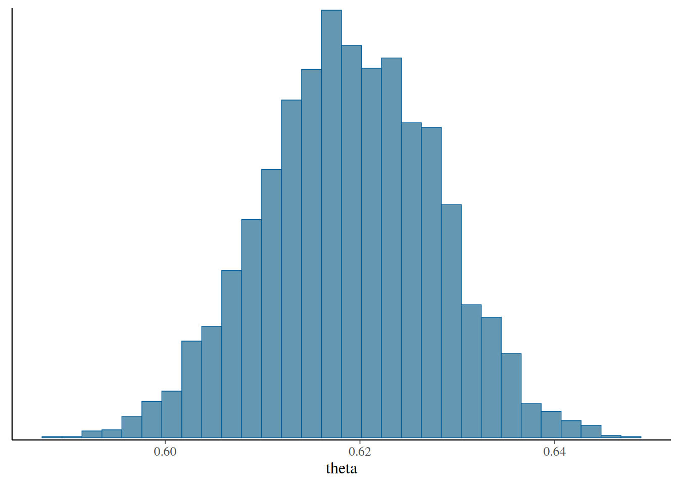
The results are similar to those in last class.
5.3 Prior Predictive Check
In Bayesian analyses, it is recommended to check both the prior and the model. This can be done by
- Prior predictive check: Simulating data from the prior distribution, and see if the simulated data fit our prior belief.
- Posterior predictive check: Simulating data from the posterior distribution, and see if the simulated data are comparable to the observed data.
We will use the following Stan code to do prior and posterior predictive checks, which has an additional generated quantity block to obtain
-
prior_theta: simulated values of \(\theta\) based on the prior distribution -
prior_ytilde: simulated data based on the prior distribution of \(\theta\) -
ytilde: simulated data based on the posterior distribution of \(\theta\)
data {
  int<lower=0> N;  // number of observations
  array[N] int<lower=0,upper=1> y;  // y
}
parameters {
  real<lower=0,upper=1> theta;  // theta parameter
}
model {
  theta ~ beta(2, 2);  // prior: Beta(2, 2)
  y ~ bernoulli(theta);  // model: Bernoulli
}
generated quantities {
  real prior_theta = beta_rng(2, 2);
  array[N] int prior_ytilde;
  array[N] int ytilde;
  for (i in 1:N) {
    ytilde[i] = bernoulli_rng(theta);
    prior_ytilde[i] = bernoulli_rng(prior_theta);
  }
}
bern_pp_mod <- cmdstan_model("stan_code/beta-bernoulli-pp.stan")
bern_pp_fit <- bern_pp_mod$sample(
Aids2_standata,
refresh = 500 # show progress every 500 iterations
)Running MCMC with 4 sequential chains...
Chain 1 Iteration: 1 / 2000 [ 0%] (Warmup)
Chain 1 Iteration: 500 / 2000 [ 25%] (Warmup)
Chain 1 Iteration: 1000 / 2000 [ 50%] (Warmup)
Chain 1 Iteration: 1001 / 2000 [ 50%] (Sampling)
Chain 1 Iteration: 1500 / 2000 [ 75%] (Sampling)
Chain 1 Iteration: 2000 / 2000 [100%] (Sampling)
Chain 1 finished in 0.9 seconds.
Chain 2 Iteration: 1 / 2000 [ 0%] (Warmup)
Chain 2 Iteration: 500 / 2000 [ 25%] (Warmup)
Chain 2 Iteration: 1000 / 2000 [ 50%] (Warmup)
Chain 2 Iteration: 1001 / 2000 [ 50%] (Sampling)
Chain 2 Iteration: 1500 / 2000 [ 75%] (Sampling)
Chain 2 Iteration: 2000 / 2000 [100%] (Sampling)
Chain 2 finished in 0.9 seconds.
Chain 3 Iteration: 1 / 2000 [ 0%] (Warmup)
Chain 3 Iteration: 500 / 2000 [ 25%] (Warmup)
Chain 3 Iteration: 1000 / 2000 [ 50%] (Warmup)
Chain 3 Iteration: 1001 / 2000 [ 50%] (Sampling)
Chain 3 Iteration: 1500 / 2000 [ 75%] (Sampling)
Chain 3 Iteration: 2000 / 2000 [100%] (Sampling)
Chain 3 finished in 0.8 seconds.
Chain 4 Iteration: 1 / 2000 [ 0%] (Warmup)
Chain 4 Iteration: 500 / 2000 [ 25%] (Warmup)
Chain 4 Iteration: 1000 / 2000 [ 50%] (Warmup)
Chain 4 Iteration: 1001 / 2000 [ 50%] (Sampling)
Chain 4 Iteration: 1500 / 2000 [ 75%] (Sampling)
Chain 4 Iteration: 2000 / 2000 [100%] (Sampling)
Chain 4 finished in 0.9 seconds.
All 4 chains finished successfully.
Mean chain execution time: 0.9 seconds.
Total execution time: 3.7 seconds.With Stan, because we obtained 4,000 prior/posterior draws (the software default) of \(\theta\), we also obtained 4,000 simulated data sets. We can see the first one, based on only the prior distribution (i.e., \(\theta\) \(\sim\) \(\text{Beta}(2, 2)\)):
bern_pp_fit$draws("prior_ytilde", format = "draws_df")[1, ] |>
    as.numeric() |>
    table()
   0    1
1005 1841
Note that the data set has more 1’s than 0’s. Our prior is weak, which means that it allows for a lot of variation in how the data would look.
The distribution of simulated data based on the prior distribution of the parameters is called the prior predictive distribution. Mathematically, we write it as
\[ P(\tilde y) = \int P(\tilde y | \theta) P(\theta) \; \mathrm{d}\theta \]
Because we have 4,000 data sets, it is not easy to visualize all individual data points. Instead, we can visualize some summary statistics of the simulated data. Here, we will choose the proportion of deaths (i.e., the mean of the variable) in each simulated data set:
bern_pp_fit$draws("prior_ytilde", format = "draws_matrix") |>
    ppd_stat(stat = "mean")
`stat_bin()` using `bins = 30`. Pick better value with `binwidth`.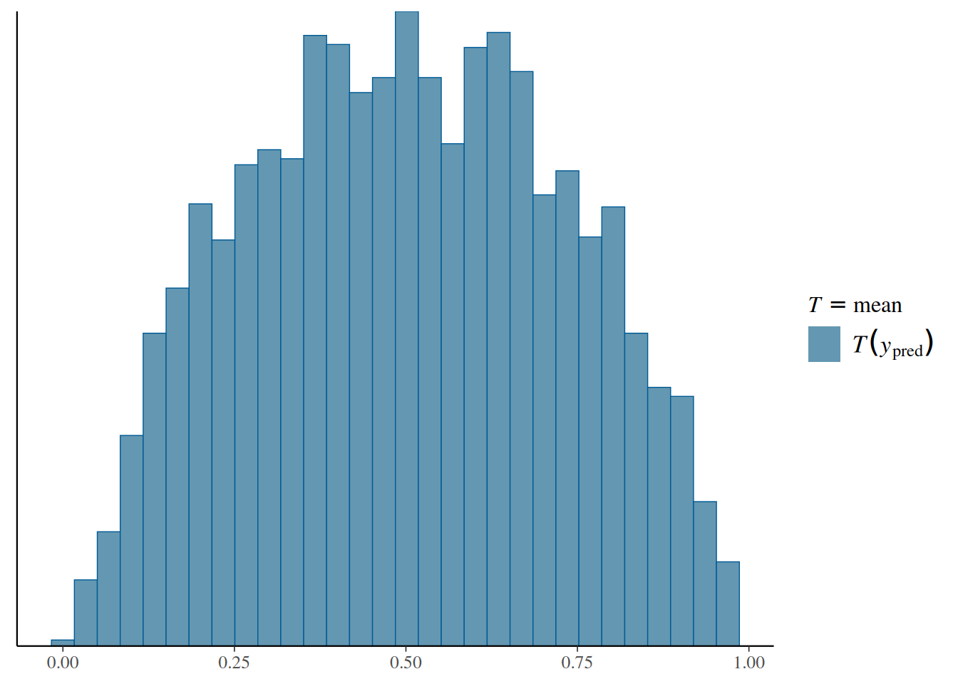
This represents our prior belief about the proportion of deaths without looking at the actual data. If this doesn’t seem to match our belief, we may want to modify our prior distribution and do the prior predictive check again, until the simulated data matches our actual prior belief.
5.4 Posterior Predictive Check
5.4.1 Check 1: Sample Mean
\[ P(\tilde y | y) = \int P(\tilde y | \theta, y) P(\theta | y) \; \mathrm{d}\theta \]
The difference here is that we use the posterior distribution \(P(\theta | y)\) instead of the prior distribution \(P(\theta)\). We can obtain the posterior predictive distribution of the death rate, and indicate the actual data in the plot:
bern_pp_fit$draws("ytilde", format = "draws_matrix") |>
    ppc_stat(y = Aids2_standata$y, stat = "mean")
`stat_bin()` using `bins = 30`. Pick better value with `binwidth`.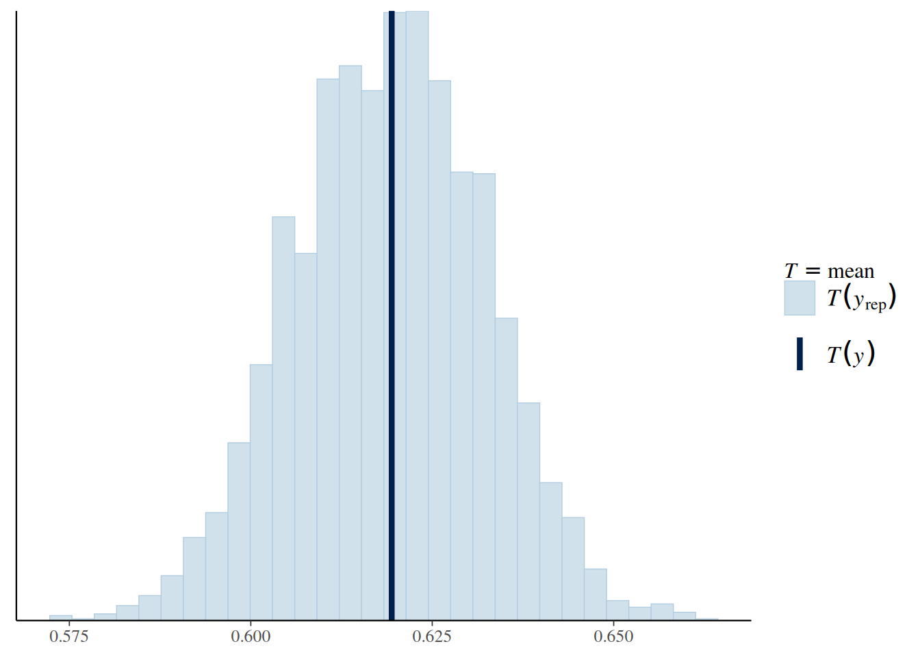
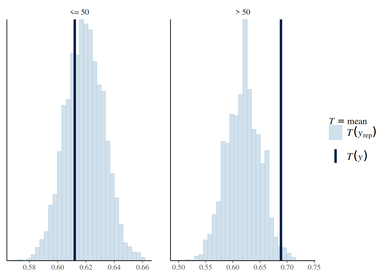
5.4.2 Check 2: Sample Mean by Age Group
# Create binary indicator of two age groups
age50 <- factor(Aids2$age > 50, labels = c("<= 50", "> 50"))
bern_pp_fit$draws("ytilde", format = "draws_matrix") |>
    ppc_stat_grouped(y = Aids2_standata$y, group = age50,stat = "mean")
`stat_bin()` using `bins = 30`. Pick better value with `binwidth`.