dag1 <- dagitty("dag{ S -> H }")
coordinates(dag1) <- list(x = c(S = 0, H = 1),
                          y = c(S = 0, H = 0))
# Plot
ggdag(dag1) + theme_dag()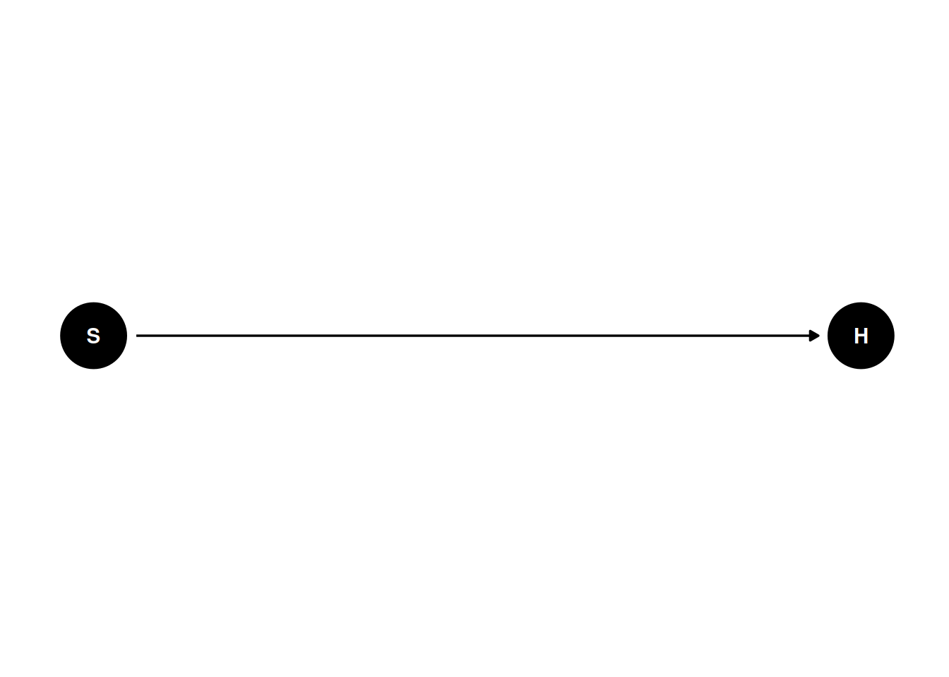
Missing data are common in many research problems. Sometimes missing data arise from design, but more commonly, data are missing for reasons that are beyond researchers’ control.
The treatment of missing data depends on the underlying causal structure (likely everything else), so you need some causal diagrams. The following examples are based on the ones in McElreath (2020, chapter 15.2). Let’s say we have a sample of students. I want to study the association between the number of hours each student studied per day (\(S\)) and the quality of the homework (\(H\)). We have the following DAG:
dag1 <- dagitty("dag{ S -> H }")
coordinates(dag1) <- list(x = c(S = 0, H = 1),
y = c(S = 0, H = 0))
# Plot
ggdag(dag1) + theme_dag()Let’s say the actual data generating model is
\[ H_i \sim N(\beta_0 + \beta_1 S_i, \sigma), \]
with \(\beta_0\) = 5, \(\beta_1\) = 1, \(\sigma\) = 0.7.
set.seed(1551)
num_obs <- 200
full_data <- data.frame(
    S = pmin(rgamma(num_obs, shape = 10, scale = 0.2), 5)
) |>
mutate(H = 5 + S + rnorm(S, sd = 0.7))ggplot(full_data, aes(x = S, y = H)) +
geom_point() +
geom_smooth(method = "lm")`geom_smooth()` using formula = 'y ~ x'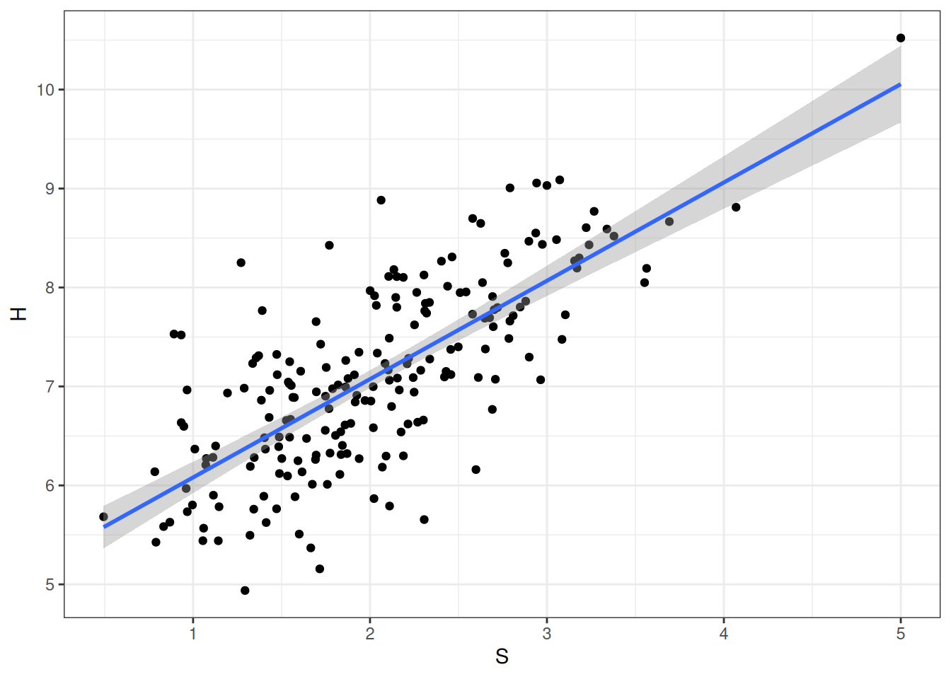
The statistical literature has generally distinguished three types of missing data mechanisms, with some confusing names: missing completely at random (MCAR), missing at random (MAR), and missing not at random (MNAR). Let’s see each of them with the corresponding causal diagram.
Let’s say all students have dogs, and somehow for some of the students, their dogs would eat their homework, producing missing data. Let \(D\) be an indicator for whether the dog ate the homework. To be consistent with the missing data literature, we set \(D\) = 0 to mean that the dog ate the homework, so that there is missing homework. When \(D\) = 1, the homework is turned in.
The impact of missing data is through two things. First, it reduces the sample size. Second, and more importantly, it can lead to a biased sample that gives non-representative estimates, compared to what you would get with the full data. Think about why polls may get election results wrong, even if they have a large sample: the sample in the pool has different characteristics from the actual voters.
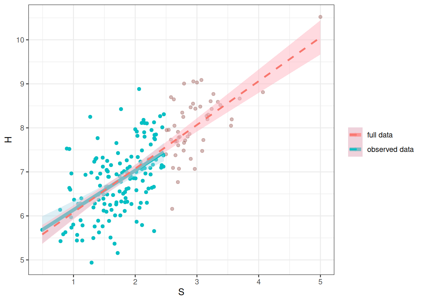
The missing data mechanism that is relatively less harmful is missing completely at random (MCAR). It means that why the data are missing—or why the dog ate the homework—happens completely on a random basis. Let H* be the observed homework variable with missing data. We have the DAG in Figure 22.3:
dag2 <- dagitty('dag{ "S" -> "H" -> "H*" ; "D" -> "H*"}')
latents(dag2) <- c("H")
coordinates(dag2) <- list(x = c(S = 0, H = 1, `H*` = 1, D = 0),
                          y = c(S = 1, H = 1, `H*` = 0, D = 0))
# Plot
ggdag(dag2) + theme_dag()
From the DAG, the association between S and H* is not confounded by D, so missing data won’t bias the coefficient.
Let’s simulate ~ 25% completely random missing data.
mcar_data <- full_data |>
    mutate(D = rbinom(num_obs, size = 1, prob = .75),
Hs = if_else(D == 1, H, NA_real_))ggplot(mcar_data) +
geom_histogram(aes(x = H, fill = "full data"), alpha = 0.5) +
geom_histogram(aes(x = Hs, fill = "observed data"), alpha = 0.5) +
labs(fill = NULL)`stat_bin()` using `bins = 30`. Pick better value with `binwidth`.
`stat_bin()` using `bins = 30`. Pick better value with `binwidth`.Warning: Removed 59 rows containing non-finite values (`stat_bin()`).ggplot(full_data, aes(x = S, y = H)) +
geom_point(aes(col = "full data"), alpha = 0.2) +
geom_point(data = mcar_data, aes(y = Hs, col = "observed data")) +
geom_smooth(data = mcar_data,
aes(y = Hs, col = "observed data"),
method = "lm", linewidth = 2, fill = "lightblue") +
geom_smooth(aes(col = "full data"),
method = "lm", alpha = 0.5, linetype = "dashed",
fill = "lightpink") +
labs(col = NULL)`geom_smooth()` using formula = 'y ~ x'Warning: Removed 59 rows containing non-finite values (`stat_smooth()`).`geom_smooth()` using formula = 'y ~ x'Warning: Removed 59 rows containing missing values (`geom_point()`).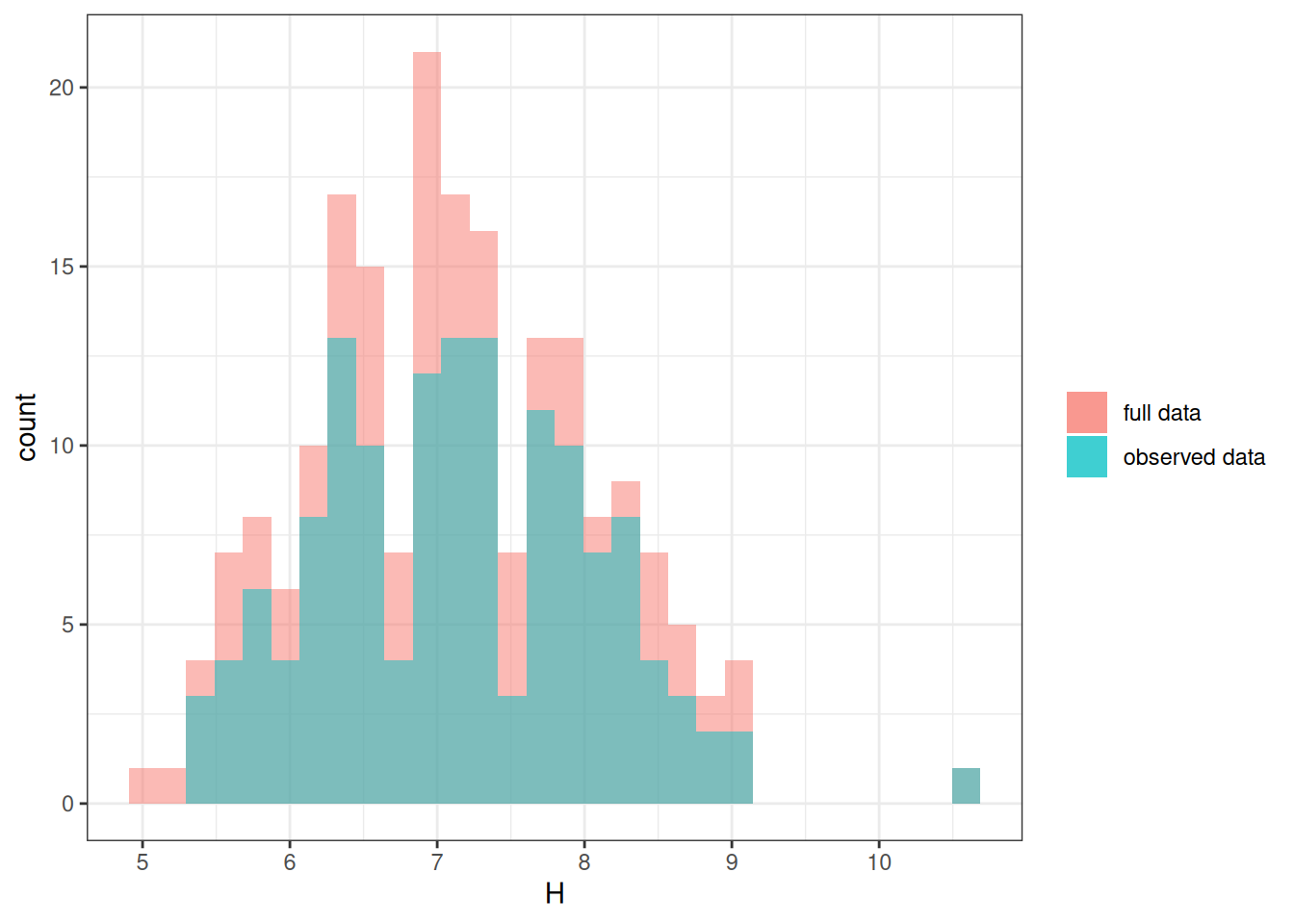
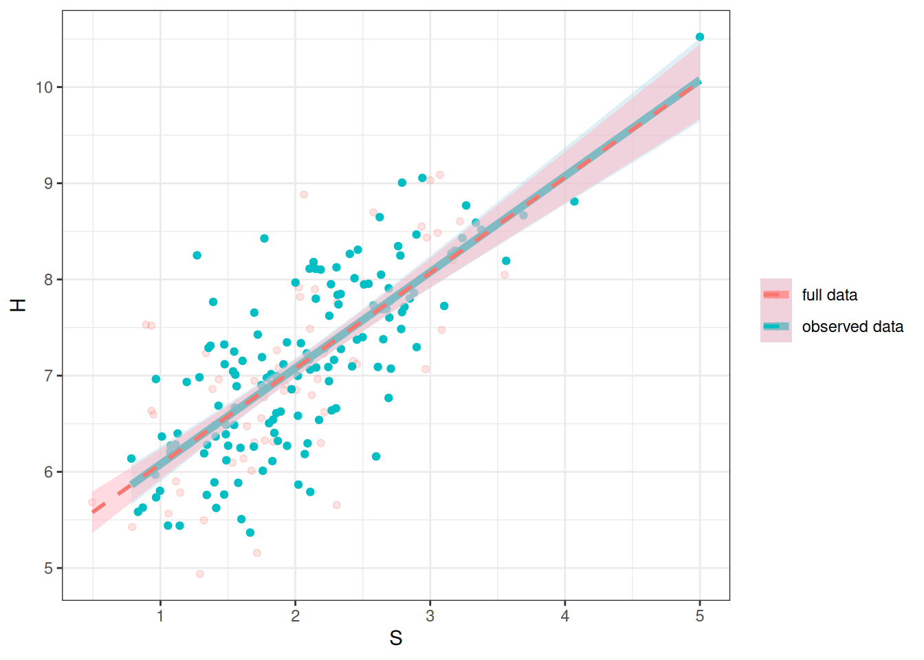
The regression line is pretty much the same as what you got with the full data; just that the uncertainty bound is a bit wider.
Now, let’s consider the situation where dogs are more dissatisfied when the students spend more time studying, and less time with them, so they are more likely to eat the homework. The term missing at random is a very confusing terminology, but it means that observed data in the model can explain the missingness. So if we include \(S\) in the model, we account for the missing data mechanism. We can see the DAG in Figure 22.5:
dag3 <- dagitty('dag{ "S" -> "H" -> "H*" ; "S" -> "D" -> "H*"}')
latents(dag3) <- c("H")
coordinates(dag3) <- list(x = c(S = 0, H = 1, `H*` = 1, D = 0),
                          y = c(S = 1, H = 1, `H*` = 0, D = 0))
# Plot
ggdag(dag3) + theme_dag()
Another way to determine whether \(S\) is sufficient to account for the missing data mechanism is to use the \(d\)-separation criteria, which you can find in the dagitty package with the dseparated() function. The goal is to find a variable set that makes \(D\) and \(H\) conditionally independent.
dseparated(dag3, "D", "H", Z = c("S")) # d-separated[1] TRUELet’s simulate some data with the dogs eating homework for the most hardworking students (or those who study too much).
mar_data <- full_data |>
    mutate(D = as.numeric(S < quantile(S, probs = .75)),
           Hs = if_else(D == 1, H, NA_real_))
As you can see in Figure 22.6, the distribution of \(H\) is now very different from that of \(H*\), but it does not distort the association between \(S\) and \(H\).
ggplot(mar_data) +
    geom_histogram(aes(x = H, fill = "full data"), alpha = 0.5) +
    geom_histogram(aes(x = Hs, fill = "observed data"), alpha = 0.5) +
    labs(fill = NULL)
`stat_bin()` using `bins = 30`. Pick better value with `binwidth`.
`stat_bin()` using `bins = 30`. Pick better value with `binwidth`.Warning: Removed 50 rows containing non-finite values (`stat_bin()`).ggplot(full_data, aes(x = S, y = H)) +
geom_point(alpha = 0.2) +
geom_point(aes(col = "full data"), alpha = 0.2) +
geom_point(data = mar_data, aes(y = Hs, col = "observed data")) +
geom_smooth(data = mar_data,
aes(y = Hs, col = "observed data"),
method = "lm", linewidth = 2, fill = "lightblue") +
geom_smooth(aes(col = "full data"),
method = "lm", alpha = 0.5, linetype = "dashed",
fill = "lightpink") +
labs(col = NULL)`geom_smooth()` using formula = 'y ~ x'Warning: Removed 50 rows containing non-finite values (`stat_smooth()`).`geom_smooth()` using formula = 'y ~ x'Warning: Removed 50 rows containing missing values (`geom_point()`).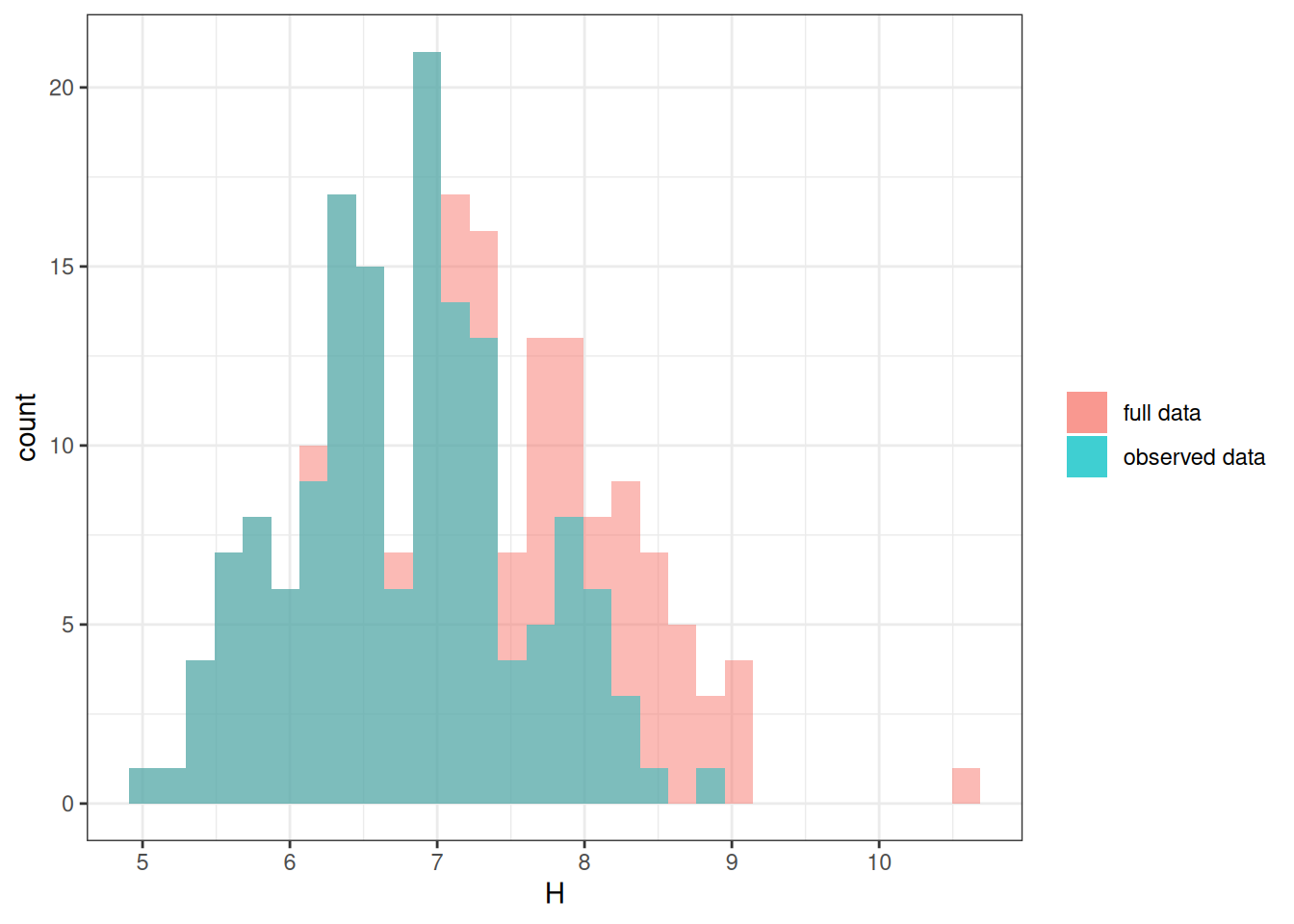
Now, let’s imagine there is an additional variable, \(X\), representing the noise level at the student’s home. As you can guess, dogs are more likely to misbehave in noisier environments, and homework quality may suffer in a noisier environment. So we have Figure 22.7.
dag4 <- dagitty('dag{ "S" -> "H" -> "H*" ; "S" -> "D" -> "H*";
                      "D" <- "X" -> "H" }')
latents(dag4) <- c("H")
coordinates(dag4) <- list(x = c(S = 0, H = 1, `H*` = 1, D = 0, X = 0.5),
                          y = c(S = 1, H = 1, `H*` = 0, D = 0, X = 0.5))
# Plot
ggdag(dag4) + theme_dag()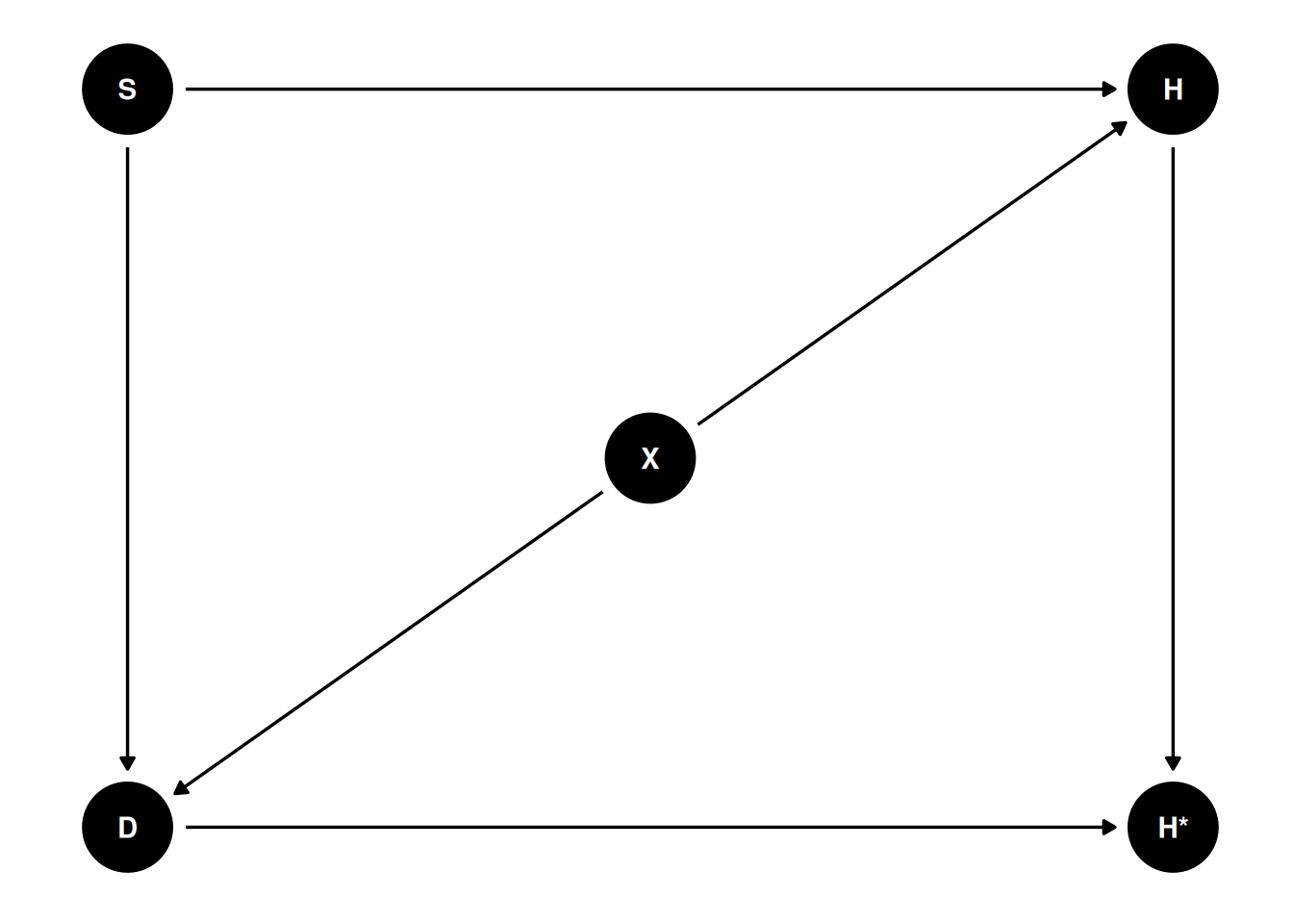
If we only include $ S$ to predict $ H*$ in our model, this mechanism is called missing not at random (MNAR). Here, even when we condition on \(S\), there is still an association between \(D\) and \(H\), due to the shared parent \(X\). We can see this in R:
dseparated(dag4, "D", "H", Z = c("S")) # not d-separated[1] FALSESo the missing data will lead to biased results. Let’s simulate some data.
ggplot(full_data2, aes(x = S, y = H)) +
    geom_point(aes(col = "full data"), alpha = 0.2) +
    geom_point(data = mnar_data1, aes(y = Hs, col = "observed data")) +
    geom_smooth(data = mnar_data1,
                aes(y = Hs, col = "observed data"),
                method = "lm", size = 2, fill = "lightblue") +
    geom_smooth(aes(col = "full data"),
                method = "lm", alpha = 0.5, linetype = "dashed",
                fill = "lightpink") +
    labs(col = NULL)
Warning: Using `size` aesthetic for lines was deprecated in ggplot2 3.4.0.
ℹ Please use `linewidth` instead.`geom_smooth()` using formula = 'y ~ x'Warning: Removed 53 rows containing non-finite values (`stat_smooth()`).`geom_smooth()` using formula = 'y ~ x'Warning: Removed 53 rows containing missing values (`geom_point()`).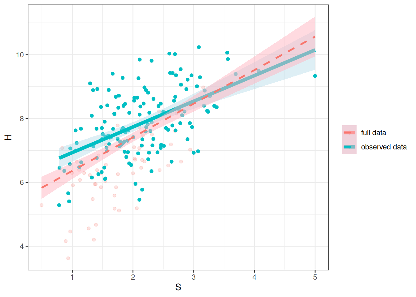
As you can see in Figure 22.8, the red line gives a biased representation of the blue line.
In this case, if we have measured \(X\), including \(X\) also in our model would give the correct result. We can check for \(d\)-separation:
dseparated(dag4, "D", "H", Z = c("S", "X")) # d-separated[1] TRUESo MNAR depends on whether our model fully accounts for the missing data mechanism. Here, it is MNAR if we do not include \(X\), but it will be MAR if we include \(X\). The following shows the results when conditioning on \(X\).
# Prediction with X added to the equation
full_data2 <- full_data2 |>
    mutate(Sres = residuals(lm(S ~ X)),
           Hres = residuals(lm(H ~ X)))
mnar_data1 <- mnar_data1 |>
    drop_na() |>
    mutate(Sres = residuals(lm(S ~ X)),
           Hres = residuals(lm(Hs ~ X)))
mnar_data1 <- cbind(
    mnar_data1,
    predict(lm(Hres ~ S, data = mnar_data1),
        newdata = mnar_data1, interval = "confidence"
    )
)ggplot(full_data2, aes(x = Sres, y = Hres)) +
geom_point(aes(col = "full data"), alpha = 0.2) +
geom_point(data = mnar_data1, aes(y = Hres, col = "observed data")) +
geom_smooth(data = mnar_data1,
aes(col = "observed data"),
method = "lm", size = 2, fill = "lightblue") +
geom_smooth(aes(col = "full data"),
method = "lm", alpha = 0.5, linetype = "dashed",
fill = "lightpink") +
labs(col = NULL, x = "S (conditioned on X)", y = "H (conditioned on X)")`geom_smooth()` using formula = 'y ~ x'
`geom_smooth()` using formula = 'y ~ x'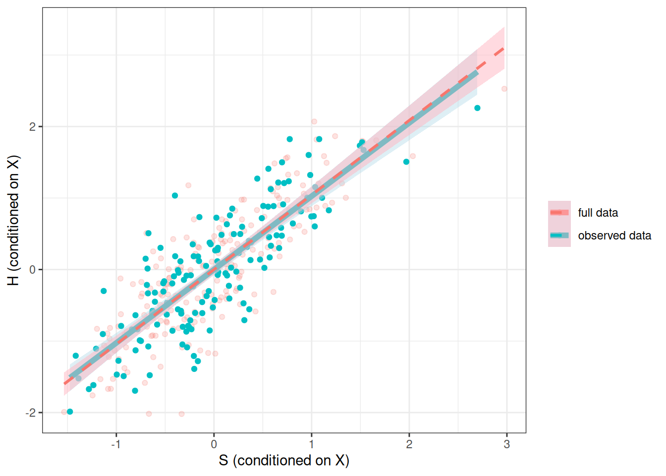
The more prototypical situation for MNAR, which is also the most problematic, is when missingness is directly related to the outcome variable, i.e., dogs like to eat bad homework.
dag5 <- dagitty('dag{ "S" -> "H" -> "H*" ; "H" -> "D" -> "H*" }')
latents(dag5) <- c("H")
coordinates(dag5) <- list(x = c(S = 0, H = 1, `H*` = 1, D = 0),
                          y = c(S = 1, H = 1, `H*` = 0, D = 0))
# Plot
ggdag(dag5) + theme_dag()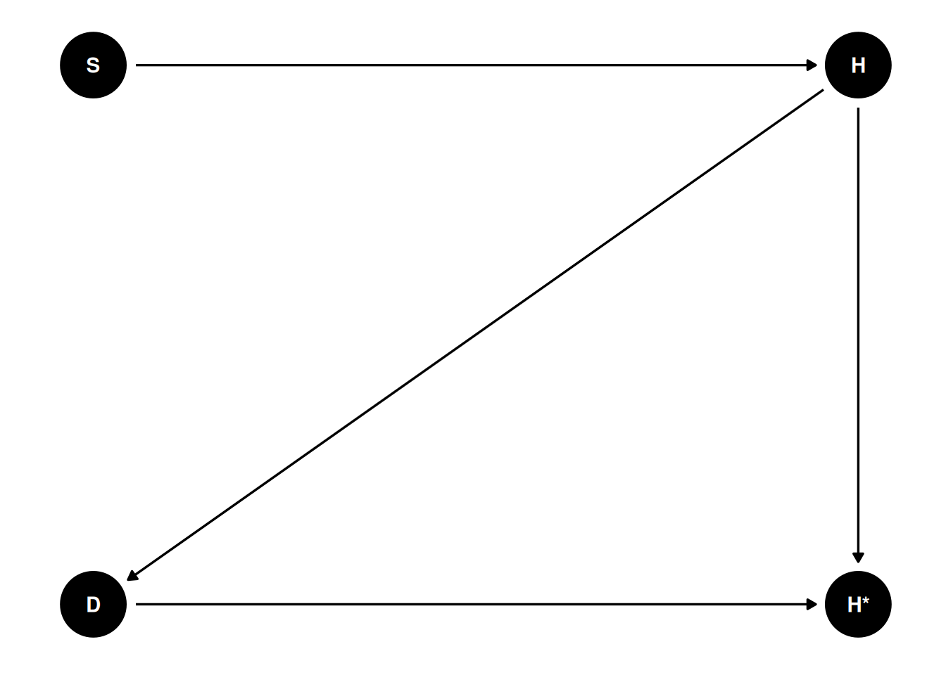
mnar_data2 <- full_data |>
    mutate(D = as.numeric(H > quantile(H, probs = .25)),
Hs = if_else(D == 1, H, NA_real_))ggplot(full_data, aes(x = S, y = H)) +
geom_point(alpha = 0.2) +
geom_point(aes(col = "full data"), alpha = 0.2) +
geom_point(data = mnar_data2, aes(y = Hs, col = "observed data")) +
geom_smooth(data = mnar_data2,
aes(y = Hs, col = "observed data"),
method = "lm", size = 2, fill = "lightblue") +
geom_smooth(aes(col = "full data"),
method = "lm", alpha = 0.5, linetype = "dashed",
fill = "lightpink") +
labs(col = NULL)`geom_smooth()` using formula = 'y ~ x'Warning: Removed 50 rows containing non-finite values (`stat_smooth()`).`geom_smooth()` using formula = 'y ~ x'Warning: Removed 50 rows containing missing values (`geom_point()`).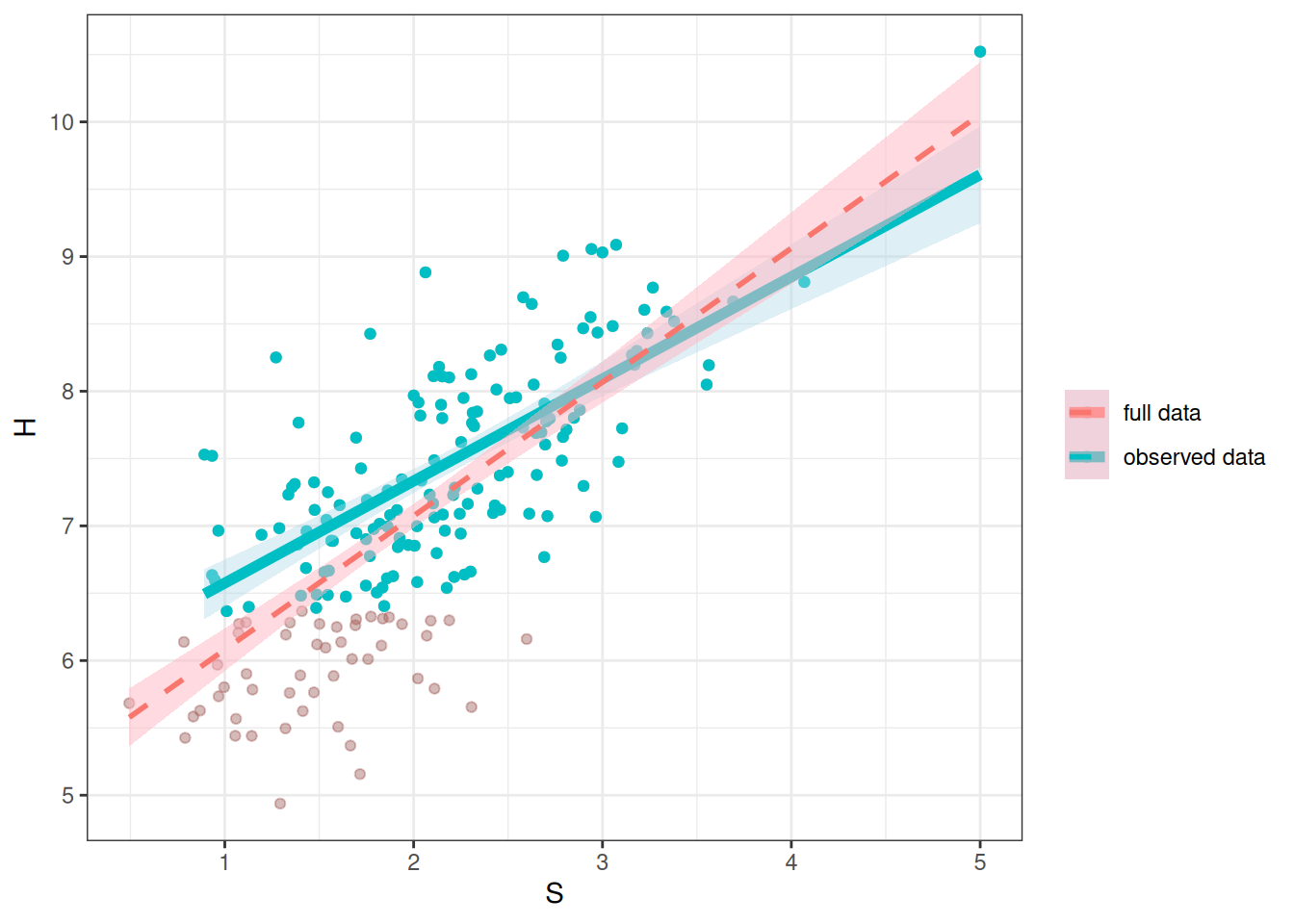
MNAR is sometimes called missing not at random or non-ignorable missingness, and as the name suggests, it refers to conditions where MAR does not hold. If you just look at the observed data, they may look very similar to the data with MAR.
Generally speaking, there are no statistical procedures distinguishing between MAR in general and MNAR.
The data come from the second edition of the book Applied Missing Data Analysis. It is from the National Institute of Mental Health Schizophrenia Collaborative Study on how treatment related to change in the severity of participants’ conditions over six weeks. This paper: https://psycnet.apa.org/record/1997-07778-004 contains more descriptions of the data.
zip_data <- here("data", "AMDA_Chapter5.zip")
if (!file.exists(zip_data)) {
    download.file("https://dl.dropboxusercontent.com/scl/fi/isztu1ee4xxm6dm5vzngc/AMDA-Chapter-5-Bayesian-Estimation-with-Missing-Data.zip?rlkey=x4onm0wj1yaktltpndkhpllgd&dl=1",
              zip_data)
}
drug_data <- read.table(
  unz(zip_data,
      "AMDA Chapter 5 - Bayesian Estimation with Missing Data/Example 5.8 - Bayes Estimation with Auxiliary Variables/drugtrial.dat"),
      col.names = c("id", "male", "drug", "severe0", "severe1",
                    "severe3", "severe6", "dropgrp", "edrop",
                    "ldrop", "dropout", "sdrop3", "sdrop6"),
na.strings = "999")rmarkdown::paged_table(drug_data)mice::md.pattern(drug_data, rotate.names = TRUE)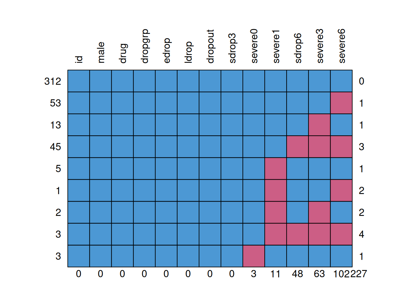
    id male drug dropgrp edrop ldrop dropout sdrop3 severe0 severe1 sdrop6
312  1    1    1       1     1     1       1      1       1       1      1
53   1    1    1       1     1     1       1      1       1       1      1
13   1    1    1       1     1     1       1      1       1       1      1
45   1    1    1       1     1     1       1      1       1       1      0
5    1    1    1       1     1     1       1      1       1       0      1
1    1    1    1       1     1     1       1      1       1       0      1
2    1    1    1       1     1     1       1      1       1       0      1
3    1    1    1       1     1     1       1      1       1       0      0
3    1    1    1       1     1     1       1      1       0       1      1
     0    0    0       0     0     0       0      0       3      11     48
    severe3 severe6
312       1       1   0
53        1       0   1
13        0       1   1
45        0       0   3
5         1       1   1
1         1       0   2
2         0       1   2
3         0       0   4
3         1       1   1
63 102 227First, consider the missing data in severe0, which consists of only three cases. In practice, this is likely not going to affect the results much. However, for pedagogical purposes, we’ll see how Bayesian handle these.
Let’s consider this plausible DAG with drug and male predicting both severe0 and its missingness (Ds0).
dag_drug1 <- dagitty(
    'dag{ drug -> s0 -> "s0*" ; male -> s0 -> "s0*";
          drug -> Ds0 -> "s0*"; male -> Ds0 -> "s0*" }'
)
latents(dag_drug1) <- c("s0")
coordinates(dag_drug1) <- list(
    x = c(drug = 0, male = 0.3, s0 = 1, `s0*` = 1, Ds0 = 0),
    y = c(drug = 0.7, male = 1, s0 = 1, `s0*` = 0, Ds0 = 0)
)
# Plot
ggdag(dag_drug1) + theme_dag()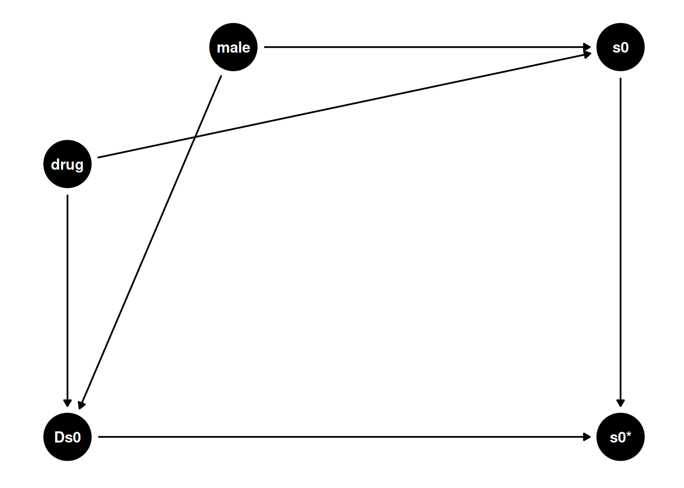
severe0.
From a Bayesian perspective, any unknown can be treated as a parameter. This includes missing data. So we can treat the missing values of severe0 as parameters, which I will call y_mis.
Here’s the Stan code
data {
  int<lower=0> N_obs;  // number of observations
  int<lower=0> N_mis;  // number of observations missing Y
  int<lower=0> p;  // number of predictors
  vector[N_obs] y_obs;  // outcome observed;
  matrix[N_obs, p] x_obs;  // predictor matrix (observed);
  matrix[N_mis, p] x_mis;  // predictor matrix (missing);
}
parameters {
  real beta0;  // regression intercept
  vector[p] beta;  // regression coefficients
  real<lower=0> sigma;  // SD of prediction error
  vector[N_mis] y_mis;  // outcome missing;
}
model {
  // model
  y_obs ~ normal_id_glm(x_obs, beta0, beta, sigma);
  y_mis ~ normal_id_glm(x_mis, beta0, beta, sigma);
  // prior
  beta0 ~ normal(0, 5);
  beta ~ normal(0, 2);
  sigma ~ student_t(4, 0, 5);
}
generated quantities {
  vector[N_obs] y_rep;  // place holder
  for (n in 1:N_obs)
    y_rep[n] = normal_rng(beta0 + dot_product(beta, x_obs[n]), sigma);
}
mr_mis <- cmdstan_model("stan_code/multiple_reg_mis.stan")Notice that the data are separated into those with severe0 observed, and those missing severe0.
# Indicator for missing `severe0`
which_mis <- which(is.na(drug_data$severe0))
which_obs <- which(!is.na(drug_data$severe0))
m1_stan <- mr_mis$sample(
    data = list(
        N_obs = length(which_obs),
        N_mis = length(which_mis),
        p = 2,
        y_obs = drug_data$severe0[which_obs],
        x_obs = drug_data[which_obs, c("drug", "male")],
        x_mis = drug_data[which_mis, c("drug", "male")]
    ),
    seed = 2222
)
Now, consider the posterior draws of y_mis
m1_stan$draws() |>
    mcmc_areas(regex_pars = "^y_mis")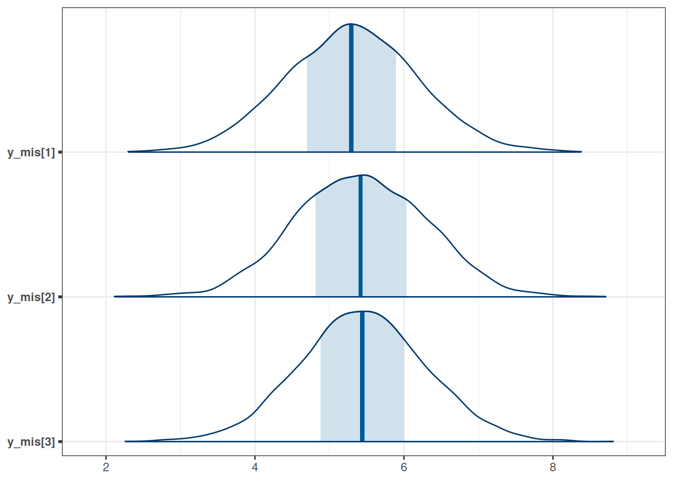
brms
The same can be done in brms with the mi() syntax:
m1_brm <- brm(severe0 | mi() ~ drug + male,
    data = drug_data,
    seed = 2234,
    file = "12_m1_brm"
)mcmc_plot(m1_brm,
type = "areas",
variable = "^Ymi",
regex = TRUE)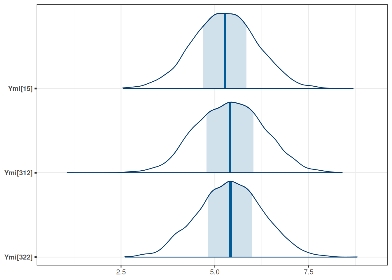
The technique of multiple imputation is a Bayesian technique widely applied in statistics. The idea is to obtain multiple draws from the posterior distributions of the missing values. For example, we can randomly obtain five draws of the three missing values:
set.seed(937)
as_draws_df(m1_stan) |>
    subset_draws(variable = "y_mis",
                 draw = sample.int(4000, 5))
Merging chains in order to subset via 'draw'.m2_brm <- brm(
bf(severe6 | mi() ~ drug + male + mi(severe0)) +
bf(severe0 | mi() ~ drug + male) +
set_rescor(FALSE),
data = drug_data,
seed = 2234,
file = "12_m2_brm"
)There are many packages for multiple imputation with different algorithms, including popular packages like mice and mdmb. Generally speaking, these packages also used the same Bayesian logic as discussed above, but employed some assumptions and techniques that make computations faster for large data sets. One possible workflow is to use these packages to perform multiple imputations, perform Bayesian analyses in each imputed data set, and then pool the results together. Below I provide an example of doing so in mice and brms.
A word of caution is needed: the algorithms in mice and related packages involve a lot of choices, and there is a full manual on using mice that you should check out before you use the package: https://stefvanbuuren.name/fimd/. While software makes sensible defaults, in my experience, when the number of variables and the proportion of missing data is large, setting up a reasonable imputation model requires a lot of careful consideration, and still, you may run into convergence issues. One thing you should make sure to do is to check for convergence of the imputation, which is very similar to checking MCMC convergence (as imputations are kind of like MCMC draws).
Another drawback of these algorithms is that, by default, they do not take into account the causal mechanism of why data are missing. Therefore, they may introduce bias due to, for example, conditioning on a collider. So you should carefully specify which variables you want to include when imputing missing data.
See this paper: https://www.tandfonline.com/doi/abs/10.1080/00273171.2014.931799 for a discussion on potential biases when including descendants of the predictors in the imputation step.
# First, obtain the default settings
imp <- mice(drug_data, visit = "monotone", maxit = 0)
Warning: Number of logged events: 2# These are the default imputation method (predictive mean matching)
imp$method id male drug severe0 severe1 severe3 severe6 dropgrp edrop ldrop
"" "" "" "pmm" "pmm" "pmm" "pmm" "" "" ""
dropout sdrop3 sdrop6
"" "" "" # We should define which variables are used to impute which variables
(pred <- imp$predictorMatrix) id male drug severe0 severe1 severe3 severe6 dropgrp edrop ldrop
id 0 1 1 1 1 1 1 1 1 1
male 1 0 1 1 1 1 1 1 1 1
drug 1 1 0 1 1 1 1 1 1 1
severe0 1 1 1 0 1 1 1 1 1 1
severe1 1 1 1 1 0 1 1 1 1 1
severe3 1 1 1 1 1 0 1 1 1 1
severe6 1 1 1 1 1 1 0 1 1 1
dropgrp 1 1 1 1 1 1 1 0 1 1
edrop 1 1 1 1 1 1 1 1 0 1
ldrop 1 1 1 1 1 1 1 1 1 0
dropout 1 1 1 1 1 1 1 1 1 1
sdrop3 1 1 1 1 1 1 1 1 1 1
sdrop6 0 0 0 0 0 0 0 0 0 0
dropout sdrop3 sdrop6
id 1 0 0
male 1 0 0
drug 1 0 0
severe0 1 0 0
severe1 1 0 0
severe3 1 0 0
severe6 1 0 0
dropgrp 1 0 0
edrop 1 0 0
ldrop 1 0 0
dropout 0 0 0
sdrop3 1 0 0
sdrop6 0 0 0# Set imputation predictors to empty (0) for the four variables
# `severe0` to `severe6`
pred[c("severe0", "severe1", "severe3", "severe6"), ] <- 0
# Use male, drug, dropout to predict missing data in severe1
pred["severe0", c("male", "drug", "dropout")] <- 1
pred["severe1", c("severe0", "male", "drug", "dropout")] <- 1
pred["severe3", c("severe0", "severe1", "male", "drug", "dropout")] <- 1
pred["severe6", c("severe0", "severe1", "severe3",
"male", "drug", "dropout")] <- 1
# Perform imputation
imp <- mice(drug_data,
m = 20, # 20 imputed data sets
predictorMatrix = pred, # which variables to impute which
# order of imputation
visit = c("severe0", "severe1", "severe3", "severe6"),
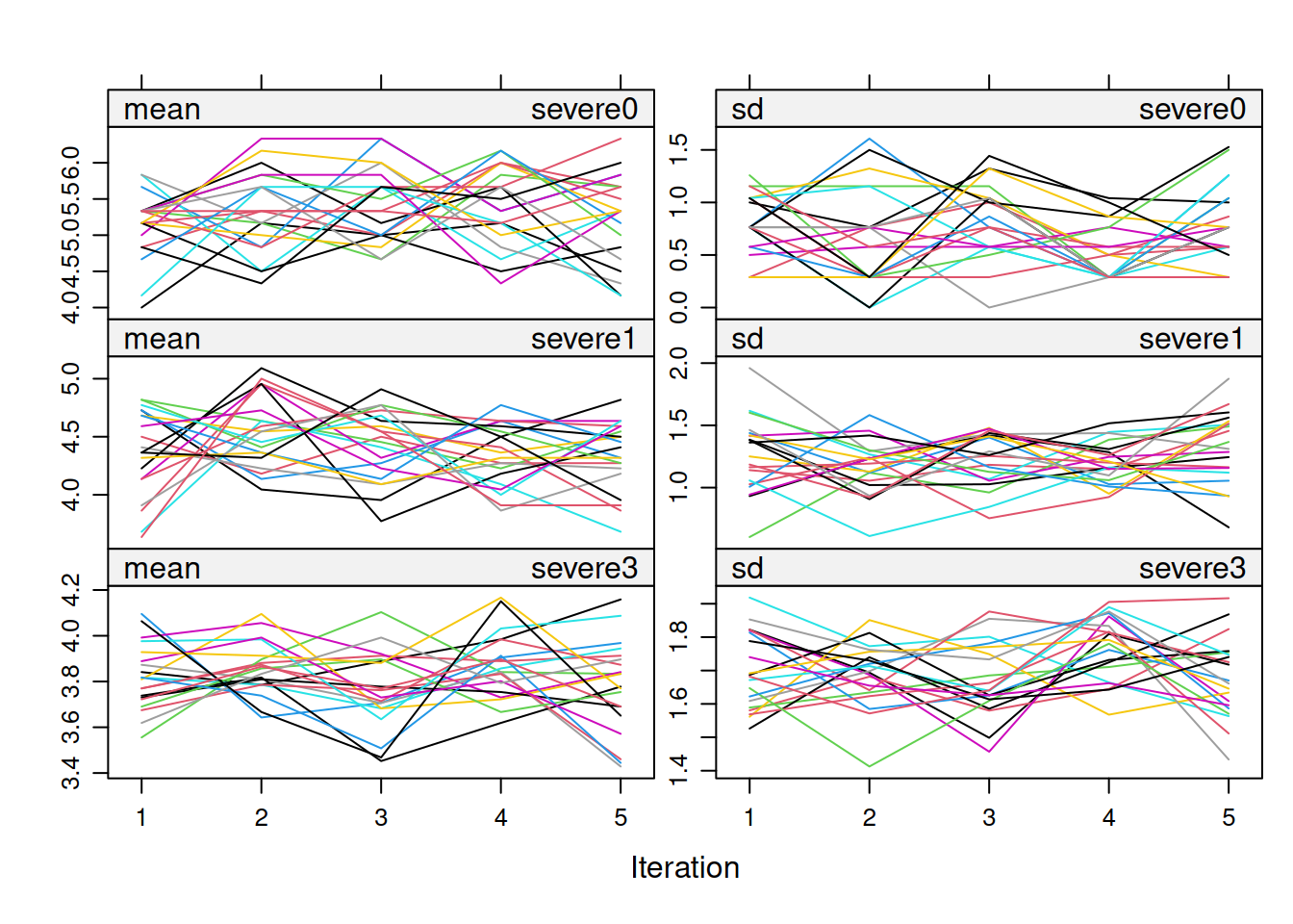
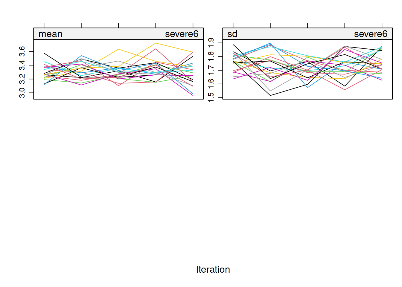
print = FALSE)Warning: Number of logged events: 100Convergence: Check the mixing of the chains.
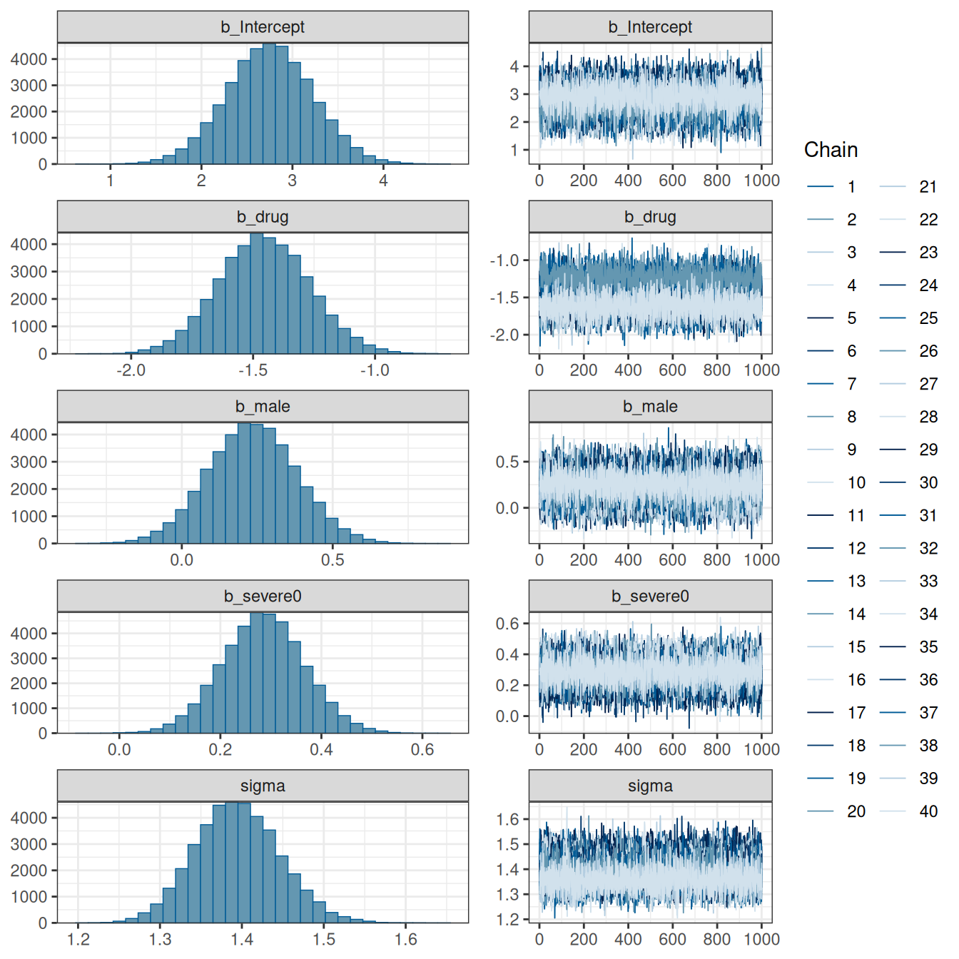
After the imputations, we can fit a Bayesian model to each of the 20 imputed data sets. brms has a handy function brm_multiple() for doing it. With 20 data sets, 2 chains each, and 2,000 iterations (1,000 warm-ups) per chain, we should get a total of 20 * 2 * 1000 = 40000 draws.
m2_imp <- brm_multiple(severe6 ~ drug + male + severe0,
    data = imp, chains = 2,
    iter = 2000,
    file = "12_m2_imp"
)
Note that because we pool estimates from different data sets, the rhat statistic is unlikely to be under 1.01, unless the imputed data sets are very similar or the missing proportion is small. On the other hand, you don’t want to see high rhat values within each imputed data set, which would indicate real convergence issues.
# Convergence with the first two chains (1st imputed data set)
as_draws_df(m2_imp) |>
    subset_draws(chain = 1:2) |>
    summarize_draws()
# And do it for each imputed data setm2_impWarning: The displayed Rhat and ESS estimates should not be trusted for
brm_multiple models. Please see ?brm_multiple for how to assess convergence of
such models. Family: gaussian
Links: mu = identity; sigma = identity
Formula: severe6 ~ drug + male + severe0
Data: imp (Number of observations: 437)
Draws: 40 chains, each with iter = 2000; warmup = 1000; thin = 1;
total post-warmup draws = 40000
Regression Coefficients:
Estimate Est.Error l-95% CI u-95% CI Rhat Bulk_ESS Tail_ESS
Intercept 2.75 0.48 1.82 3.68 1.07 336 1844
drug -1.45 0.19 -1.81 -1.09 1.21 129 447
male 0.23 0.15 -0.05 0.53 1.10 249 1081
severe0 0.29 0.08 0.13 0.45 1.05 442 2553
Further Distributional Parameters:
Estimate Est.Error l-95% CI u-95% CI Rhat Bulk_ESS Tail_ESS
sigma 1.39 0.05 1.30 1.50 1.09 264 964
Draws were sampled using sample(hmc). For each parameter, Bulk_ESS
and Tail_ESS are effective sample size measures, and Rhat is the potential
scale reduction factor on split chains (at convergence, Rhat = 1).plot(m2_imp)