17 Hamiltonian Monte Carlo

A more recent development in MCMC is the development of algorithms under the umbrella of Hamiltonian Monte Carlo or hybrid Monte Carlo (HMC). The algorithm is a bit complex, and my goal is to help you develop some intuition of the algorithm, hopefully, enough to help you diagnose the Markov chains.

It produces simulation samples that are much less correlated, meaning that if you get 10,000 samples from Metropolis and 10,000 samples from HMC, HMC generally provides a much higher effective sample size (ESS).
It does not require conjugate priors
When there is a problem in convergence, HMC tends to raise a clear red flag, meaning it goes really, really wrong.

So now, how does HMC work? First, consider a two-dimensional posterior below, which is the posterior of $(\mu, \sigma^2)$ from a normal model.

Code

ybar <- 3.096129
s2y <- 1.356451
n <- 31
# Hyperparameters
mu_0 <- 5
sigma2_0 <- 1
kappa_0 <- 1 / 10^2
nu_0 <- 1
# Joint log density
lp_mu_sigma <- function(mu, sigma2) {
    kappa_n <- kappa_0 + n
    mu_n <- (kappa_0 * mu_0 + n * ybar) / kappa_n
    nu_n <- nu_0 + n
    sigma2_n <- (nu_0 * sigma2_0 + (n - 1) * s2y +
        kappa_0 * n / kappa_n * (ybar - mu_0)^2) / nu_n
    log_dens <- -(mu - mu_n)^2 / 2 / sigma2 * kappa_n +
        (-nu_n / 2 - 1) * log(sigma2) +
        (-nu_n * sigma2_n / 2 / sigma2)
    log_dens[is.nan(log_dens)] <- -Inf
    log_dens
}

num_gridpoints <- 51
mu_grid <- seq(2, to = 4, length.out = num_gridpoints)
sigma2_grid <- seq(0.5, to = 4.5, length.out = num_gridpoints)
grid_density <- exp(outer(mu_grid,
    Y = sigma2_grid,
    FUN = lp_mu_sigma
))
surf1 <- plot_ly(
    x = ~sigma2_grid, y = ~mu_grid, z = ~grid_density,
    type = "surface"
)

surf1

Figure 17.1: Joint posterior of $(\mu, \sigma^2)$ from a normal model.

The HMC algorithm improves from the Metropolis algorithm by simulating smart proposal values. It does so by using the gradient of the logarithm of the posterior density. Let’s first take the log of the joint density:

Code

grid_logdensity <- outer(mu_grid,
    Y = sigma2_grid,
    FUN = lp_mu_sigma
)
surf2 <- plot_ly(
    x = ~sigma2_grid, y = ~mu_grid, z = ~grid_logdensity,
    type = "surface"
)

surf2

Figure 17.2: Gradient of $(\mu, \sigma^2)$ from a normal model.

Now, flip it upside-down.

Code

grid_minuslogdensity <- - outer(mu_grid,
    Y = sigma2_grid,
    FUN = lp_mu_sigma
)
surf3 <- plot_ly(
    x = ~sigma2_grid, y = ~mu_grid, z = ~grid_minuslogdensity,
    type = "surface"
)

surf3

Figure 17.3: "Flipped" gradient of $(\mu, \sigma^2)$ from a normal model.

Imagine placing a marble on the above surface. With gravity, it is natural that the marble will have a tendency to move to the bottom of the surface. If you place the marble in a higher location, it will have a higher potential energy and tends to move faster towards the bottom, because that energy converts to a larger kinetic energy. If you place it close to the bottom, it will tend to move slower.

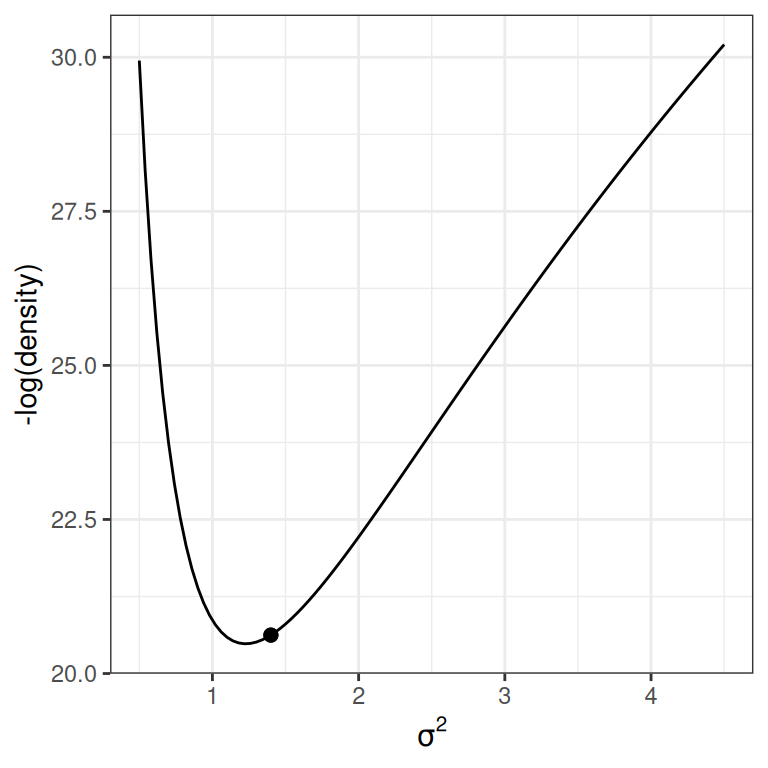
For simplicity, let’s consider just one dimension with the following picture:

Code

lp_sigma <- function(sigma2) {
    kappa_n <- kappa_0 + n
    nu_n <- nu_0 + n
    sigma2_n <- (nu_0 * sigma2_0 + (n - 1) * s2y +
        kappa_0 * n / kappa_n * (ybar - mu_0)^2) / nu_n
    log_dens <- (-nu_n / 2 - 1) * log(sigma2) +
        (-nu_n * sigma2_n / 2 / sigma2)
    log_dens[is.nan(log_dens)] <- -Inf
    log_dens
}
p2 <- ggplot(data = data.frame(x = c(0.5, 4.5)), aes(x = x)) +
    stat_function(fun = function(x) - lp_sigma(x)) +
    labs(x = expression(sigma^2),
         y = "-log(density)")
p2 +
    geom_point(
        x = 0.6, y = -lp_sigma(0.6),
        size = 2
    )
p2 +
    geom_point(
        x = 1.4, y = -lp_sigma(1.4),
        size = 2
    )

For the graph on the left, the marble (represented as a dot) has high potential energy and should quickly go down to the bottom; on the right, the marble has low potential energy and should move less fast.

If the sampler is near the bottom (i.e., the point with high posterior density), it tends to stay there.

But we don’t want the marble to stay at the bottom without moving; otherwise, all our posterior draws will be just the posterior mode. In HMC, it moves the marble with a push, called momentum. The direction and the magnitude of the momentum will be randomly simulated, usually from a normal distribution. If the momentum is large, it should travel farther away; however, it also depends on the gradient, which is the slope in a one-dimension case.

HMC generates a proposed value by simulating the motion of an object on a surface, based on an initial momentum with a random magnitude and direction, and locating the object after a fixed amount of time.

At the beginning of a trajectory, the marble has a certain amount of kinetic and potential energy, and the sum is the total amount of energy, called the Hamiltonian. Based on the conservation of energy, at any point in the motion, the Hamiltonian should remain constant.

The following shows the trajectory of a point starting at 2, with a random momentum of 0.5 in the positive direction.

Figure 17.5: Animation of HMC trajectory (momentum to the right)

This one has the same starting value, with a random momentum of 0.5 in the negative direction.

Figure 17.6: Animation of HMC trajectory (momentum to the left)

17.1 Leapfrog Integrator

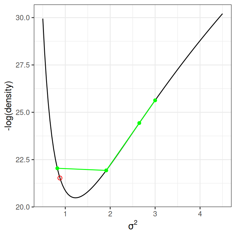
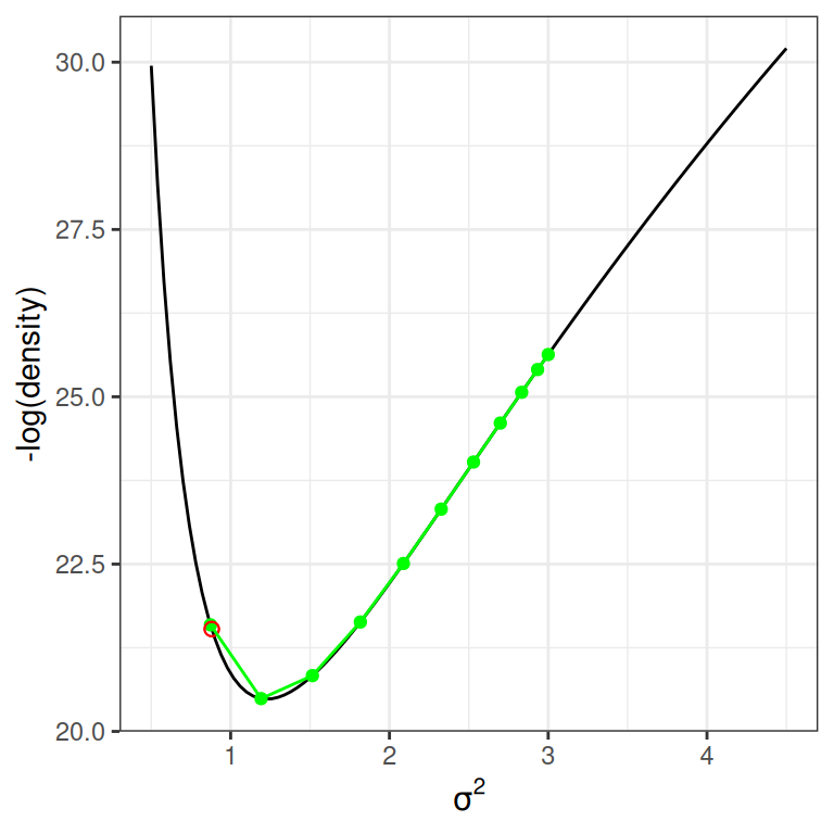
To simulate the marble’s motion, one needs to solve a system of differential equations, which is not an easy task. A standard method is the so-called leapfrog integrator, which discretizes a unit of time into $L$ steps. The following shows how it approximates the motion using $L$ = 3 and $L$ = 10 steps. The red dot is the target. As can be seen, larger $L$ simulates the motion more accurately.

Code

num_steps <- 3
leapfrog_df <- cbind(
    leapfrog_step(3, rho = -0.5, num_steps = num_steps),
    step = 0:num_steps
)
final_x <- leapfrog_step(3, rho = -0.5, num_steps = 1000)[1001, 1]
p2 + geom_point(
    data = leapfrog_df,
    aes(x = x, y = -lp_sigma(x)), col = "green"
) +
    geom_point(
        x = final_x, y = -lp_sigma(final_x),
        col = "red", size = 2, shape = 21
    ) +
    geom_path(
        data = leapfrog_df,
        aes(x = x, y = -lp_sigma(x)), col = "green"
    )
num_steps <- 10
leapfrog_df <- cbind(
    leapfrog_step(3, rho = -0.5, num_steps = num_steps),
    step = 0:num_steps
)
p2 + geom_point(
    data = leapfrog_df,
    aes(x = x, y = -lp_sigma(x)), col = "green"
) +
    geom_point(
        x = final_x, y = -lp_sigma(final_x),
        col = "red", size = 2, shape = 21
    ) +
    geom_path(
        data = leapfrog_df,
        aes(x = x, y = -lp_sigma(x)), col = "green"
    )

Suppose the simulated trajectory differs from the true trajectory by a certain threshold, like the one on the left. In that case, it is called a divergent transition, in which case the proposed value should not be trusted. In software like STAN, it will print out a warning about that. When the number of divergent transitions is large, one thing to do is increase $L$. If that does not help, it may indicate difficulty in a high-dimensional model, and reparameterization may be needed.

For more information on HMC, go to https://mc-stan.org/docs/reference-manual/mcmc.html. You can also find some sample R code at http://www.stat.columbia.edu/~gelman/book/software.pdf.

17.2 The No-U-Turn Sampler (NUTS)

Although HMC is more efficient by generating smarter proposal values, one performance bottleneck is that the motion sometimes takes a U-turn, like in some graphs above, in which the marble goes up (right) and then goes down (left), and eventually may stay in a similar location. The improvement of NUTS is that it uses a binary search tree that simulates both the forward and backward trajectory. The algorithm is complex, but to my understanding, it achieves two purposes: (a) finding the path that avoids a U-turn and (b) selecting an appropriate number of leapfrog steps, $L$. When each leapfrog step moves slowly, the search process may take a long time. With NUTS, one can control the maximum depth of the search tree.

See https://mc-stan.org/docs/reference-manual/mcmc.html#hmc-algorithm-parameters for more information on NUTS.

# Hamiltonian Monte Carlo ```{r} #| include: false comma <- function(x, digits = 2L) format(x, digits = digits, big.mark = ",") library(ggplot2) theme_set(theme_bw() + theme(panel.grid.major.y = element_line(color = "grey92"))) library(plotly) ``` A more recent development in MCMC is the development of algorithms under the umbrella of *Hamiltonian Monte Carlo* or *hybrid Monte Carlo* (HMC). The algorithm is a bit complex, and my goal is to help you develop some intuition of the algorithm, hopefully, enough to help you diagnose the Markov chains. 1. It produces simulation samples that are much less correlated, meaning that if you get 10,000 samples from Metropolis and 10,000 samples from HMC, HMC generally provides a much higher effective sample size (ESS). 2. It does not require conjugate priors 3. When there is a problem in convergence, HMC tends to raise a clear red flag, meaning it goes really, really wrong. So now, how does HMC work? First, consider a two-dimensional posterior below, which is the posterior of $(\mu, \sigma^2)$ from a normal model. ```{r} #| code-fold: true ybar <- 3.096129 s2y <- 1.356451 n <- 31 # Hyperparameters mu_0 <- 5 sigma2_0 <- 1 kappa_0 <- 1 / 10^2 nu_0 <- 1 # Joint log density lp_mu_sigma <- function(mu, sigma2) { kappa_n <- kappa_0 + n mu_n <- (kappa_0 * mu_0 + n * ybar) / kappa_n nu_n <- nu_0 + n sigma2_n <- (nu_0 * sigma2_0 + (n - 1) * s2y + kappa_0 * n / kappa_n * (ybar - mu_0)^2) / nu_n log_dens <- -(mu - mu_n)^2 / 2 / sigma2 * kappa_n + (-nu_n / 2 - 1) * log(sigma2) + (-nu_n * sigma2_n / 2 / sigma2) log_dens[is.nan(log_dens)] <- -Inf log_dens } num_gridpoints <- 51 mu_grid <- seq(2, to = 4, length.out = num_gridpoints) sigma2_grid <- seq(0.5, to = 4.5, length.out = num_gridpoints) grid_density <- exp(outer(mu_grid, Y = sigma2_grid, FUN = lp_mu_sigma )) surf1 <- plot_ly( x = ~sigma2_grid, y = ~mu_grid, z = ~grid_density, type = "surface" ) ``` ::: {.content-visible when-format="html"} ```{r} #| label: fig-normal-posterior #| fig-cap: Joint posterior of $(\mu, \sigma^2)$ from a normal model. #| fig-asp: 1 surf1 ``` ::: ```{r} #| include: false save_image(surf1, "images/surf1.png") ``` ::: {.content-visible when-format="pdf"} ![Joint posterior of $(\mu, \sigma^2)$ from a normal model.](images/surf1.png){#fig-normal-posterior} ::: The HMC algorithm improves from the Metropolis algorithm by simulating smart proposal values. It does so by using the *gradient* of the logarithm of the posterior density. Let's first take the log of the joint density: ```{r} #| code-fold: true grid_logdensity <- outer(mu_grid, Y = sigma2_grid, FUN = lp_mu_sigma ) surf2 <- plot_ly( x = ~sigma2_grid, y = ~mu_grid, z = ~grid_logdensity, type = "surface" ) ``` ::: {.content-visible when-format="html"} ```{r} #| label: fig-normal-gradient #| fig-cap: Gradient of $(\mu, \sigma^2)$ from a normal model. #| fig-asp: 1 surf2 ``` ::: ```{r} #| include: false save_image(surf2, "images/surf2.png") ``` ::: {.content-visible when-format="pdf"} ![Gradient of $(\mu, \sigma^2)$ from a normal model.](images/surf1.png){#fig-normal-gradient} ::: Now, flip it upside-down. ```{r} #| code-fold: true grid_minuslogdensity <- - outer(mu_grid, Y = sigma2_grid, FUN = lp_mu_sigma ) surf3 <- plot_ly( x = ~sigma2_grid, y = ~mu_grid, z = ~grid_minuslogdensity, type = "surface" ) ``` ::: {.content-visible when-format="html"} ```{r} #| label: fig-normal-negative-gradient #| fig-cap: \"Flipped\" gradient of $(\mu, \sigma^2)$ from a normal model. #| fig-asp: 1 surf3 ``` ::: ```{r} #| include: false save_image(surf3, "images/surf3.png") ``` ::: {.content-visible when-format="pdf"} !["Flipped" gradient of $(\mu, \sigma^2)$ from a normal model.](images/surf1.png){#fig-normal-negative-gradient} ::: Imagine placing a marble on the above surface. With gravity, it is natural that the marble will have a tendency to move to the bottom of the surface. If you place the marble in a higher location, it will have a higher *potential energy* and tends to move faster towards the bottom, because that energy converts to a larger *kinetic energy*. If you place it close to the bottom, it will tend to move slower. For simplicity, let's consider just one dimension with the following picture: ```{r} #| code-fold: true #| label: fig-posterior-sigma #| layout-ncol: 2 #| fig-width: 4 #| fig-asp: 1 #| fig-cap: Marginal log posterior distribution of $\sigma^2$. #| fig-subcap: #| - High potential energy #| - Low potential energy lp_sigma <- function(sigma2) { kappa_n <- kappa_0 + n nu_n <- nu_0 + n sigma2_n <- (nu_0 * sigma2_0 + (n - 1) * s2y + kappa_0 * n / kappa_n * (ybar - mu_0)^2) / nu_n log_dens <- (-nu_n / 2 - 1) * log(sigma2) + (-nu_n * sigma2_n / 2 / sigma2) log_dens[is.nan(log_dens)] <- -Inf log_dens } p2 <- ggplot(data = data.frame(x = c(0.5, 4.5)), aes(x = x)) + stat_function(fun = function(x) - lp_sigma(x)) + labs(x = expression(sigma^2), y = "-log(density)") p2 + geom_point( x = 0.6, y = -lp_sigma(0.6), size = 2 ) p2 + geom_point( x = 1.4, y = -lp_sigma(1.4), size = 2 ) ``` For the graph on the left, the marble (represented as a dot) has high potential energy and should quickly go down to the bottom; on the right, the marble has low potential energy and should move less fast. ::: {.callout-note} If the sampler is near the bottom (i.e., the point with high posterior density), it tends to stay there. ::: But we don't want the marble to stay at the bottom without moving; otherwise, all our posterior draws will be just the posterior mode. In HMC, it moves the marble with a push, called *momentum*. The direction and the magnitude of the momentum will be randomly simulated, usually from a normal distribution. If the momentum is large, it should travel farther away; however, it also depends on the *gradient*, which is the slope in a one-dimension case. ::: {.callout-note} HMC generates a proposed value by simulating the motion of an object on a surface, based on an initial momentum with a random magnitude and direction, and locating the object after a fixed amount of time. ::: At the beginning of a trajectory, the marble has a certain amount of kinetic and potential energy, and the sum is the total amount of energy, called the *Hamiltonian*. Based on the conservation of energy, at any point in the motion, the Hamiltonian should remain constant. ```{r} #| include: false leapfrog_step <- function(x, rho, num_steps, eps = 1 / num_steps) { out <- data.frame(x = rep(NA, num_steps + 1), rho = rep(NA, num_steps + 1)) out[1, ] <- c(x, rho) kappa_n <- kappa_0 + n nu_n <- nu_0 + n sigma2_n <- (nu_0 * sigma2_0 + (n - 1) * s2y + kappa_0 * n / kappa_n * (ybar - mu_0)^2) / nu_n for (i in seq_len(num_steps)) { rho <- rho - eps / 2 * ((nu_n / 2 + 1) / x - nu_n * sigma2_n / 2 / x^2) x <- x + eps * rho rho <- rho - eps / 2 * ((nu_n / 2 + 1) / x - nu_n * sigma2_n / 2 / x^2) out[i + 1, ] <- c(x, rho) } out } ``` ::: {.content-visible when-format="html"} The following shows the trajectory of a point starting at 2, with a random momentum of 0.5 in the positive direction. ```{r} #| echo: false #| eval: !expr '!file.exists("images/hmc1.gif")' library(gganimate) num_steps <- 50 leapfrog_steps <- leapfrog_step(2, rho = 0.5, num_steps = num_steps) p_animate <- p2 + geom_point( data = cbind(leapfrog_steps, step = 0:num_steps), aes(x = x, y = -lp_sigma(x)) ) + labs(x = expression(sigma^2), y = "-log(density)") + transition_time(step) animate(p_animate, nframes = num_steps + 1, fps = num_steps / 2, renderer = gifski_renderer(), end_pause = 10 ) anim_save("images/hmc1.gif") ``` ![Animation of HMC trajectory (momentum to the right)](images/hmc1.gif){#fig-momentum-1} This one has the same starting value, with a random momentum of 0.5 in the *negative* direction. ```{r} #| echo: false #| eval: !expr '!file.exists("images/hmc2.gif")' library(gganimate) num_steps <- 50 leapfrog_steps <- leapfrog_step(2, rho = -0.5, num_steps = num_steps) p_animate <- p2 + geom_point( data = cbind(leapfrog_steps, step = 0:num_steps), aes(x = x, y = -lp_sigma(x)) ) + labs(x = expression(sigma^2), y = "-log(density)") + transition_time(step) animate(p_animate, nframes = num_steps + 1, fps = num_steps / 2, renderer = gifski_renderer(), end_pause = 10 ) anim_save("images/hmc2.gif") ``` ![Animation of HMC trajectory (momentum to the left)](images/hmc2.gif){#fig-momentum-2} ::: ## Leapfrog Integrator To simulate the marble's motion, one needs to solve a system of differential equations, which is not an easy task. A standard method is the so-called *leapfrog* integrator, which discretizes a unit of time into $L$ steps. The following shows how it approximates the motion using $L$ = 3 and $L$ = 10 steps. The red dot is the target. As can be seen, larger $L$ simulates the motion more accurately. ```{r} #| code-fold: true #| label: fig-posterior-sigma-leapfrog #| layout-ncol: 2 #| fig-width: 4 #| fig-asp: 1 #| fig-cap: Simulated motion using the leapfrog integrator. #| fig-subcap: #| - 3 steps #| - 10 steps num_steps <- 3 leapfrog_df <- cbind( leapfrog_step(3, rho = -0.5, num_steps = num_steps), step = 0:num_steps ) final_x <- leapfrog_step(3, rho = -0.5, num_steps = 1000)[1001, 1] p2 + geom_point( data = leapfrog_df, aes(x = x, y = -lp_sigma(x)), col = "green" ) + geom_point( x = final_x, y = -lp_sigma(final_x), col = "red", size = 2, shape = 21 ) + geom_path( data = leapfrog_df, aes(x = x, y = -lp_sigma(x)), col = "green" ) num_steps <- 10 leapfrog_df <- cbind( leapfrog_step(3, rho = -0.5, num_steps = num_steps), step = 0:num_steps ) p2 + geom_point( data = leapfrog_df, aes(x = x, y = -lp_sigma(x)), col = "green" ) + geom_point( x = final_x, y = -lp_sigma(final_x), col = "red", size = 2, shape = 21 ) + geom_path( data = leapfrog_df, aes(x = x, y = -lp_sigma(x)), col = "green" ) ``` Suppose the simulated trajectory differs from the true trajectory by a certain threshold, like the one on the left. In that case, it is called a *divergent transition*, in which case the proposed value should not be trusted. In software like STAN, it will print out a warning about that. When the number of divergent transitions is large, one thing to do is increase $L$. If that does not help, it may indicate difficulty in a high-dimensional model, and reparameterization may be needed. For more information on HMC, go to <https://mc-stan.org/docs/reference-manual/mcmc.html>. You can also find some sample R code at <http://www.stat.columbia.edu/~gelman/book/software.pdf>. ## The No-U-Turn Sampler (NUTS) Although HMC is more efficient by generating smarter proposal values, one performance bottleneck is that the motion sometimes takes a U-turn, like in some graphs above, in which the marble goes up (right) and then goes down (left), and eventually may stay in a similar location. The improvement of NUTS is that it uses a binary search tree that simulates both the forward and backward trajectory. The algorithm is complex, but to my understanding, it achieves two purposes: (a) finding the path that avoids a U-turn and (b) selecting an appropriate number of leapfrog steps, $L$. When each leapfrog step moves slowly, the search process may take a long time. With NUTS, one can control the maximum *depth* of the search tree. See <https://mc-stan.org/docs/reference-manual/mcmc.html#hmc-algorithm-parameters> for more information on NUTS.