13  Causal Inference

Causal inference is an important topic in statistics, but it also has a complicated history with statistics. Early-day statisticians saw causality as a taboo such that researchers were discouraged from drawing any causal conclusions in nonexperimental research. In the past few decades, much progress has been made on causal inference in epidemiology, computer science, and statistics, with several frameworks proposed and many tools developed for experimental and nonexperimental data.¹ This note will introduce the causal diagram framework for encoding causal assumptions, which can be used to guide analysis for drawing causal conclusions. The goal is to give you some basic ideas so that you can learn more from other sources, such as the book Causality by Pearl and the book Causal Inference for Statistics, Social, and Biomedical Sciences: An Introduction by Imbens and Rubin.

Two prominent frameworks for causal inference are

1. Structural causal model, which uses tools such as DAGs and \(d\)-separation, is thoroughly described in the book Causality by Pearl, and
2. Potential outcome model, which is thoroughly described in the book Causal Inference for Statistics, Social, and Biomedical Sciences: An Introduction by Imbens and Rubin.

In this note, we will draw on both frameworks.

What is Causal Inference?

Causal inference is the process of determining the causal effect of one variable on another, based on data and causal assumptions. Two common ways of interpreting a causal effect are (a) intervention: how \(Y\) will change if \(X\) is manipulated to be \(x\); (b) counterfactual: what would \(Y\) be if \(X\) were set to \(x\).

13.1 Potential Outcomes

Consider a binary treatment variable. For each individual, there are two potential outcomes: one if they receive the treatment (T = 1) and one if they do not (T = 0). Here is a hypothetical data set of a new drug for improving statistics knowledge, with the treatment condition receiving the drug and the control condition receiving a placebo:

po_dat <- data.frame(
    person = c(1, 2, 3, 4, 5, 6, 7, 8),
    attitude = c(4, 7, 3, 9, 5, 6, 8, 2),
    treat = c(75, 80, 70, 90, 85, 82, 95, 78),
    control = c(70, 88, 75, 92, 82, 85, 90, 78)
)
knitr::kable(po_dat,
    col.names = c("Person", "Math Attitude", "Y (if T = 1)", "Y (if T = 0)"))

Person	Math Attitude	Y (if T = 1)	Y (if T = 0)
1	4	75	70
2	7	80	88
3	3	70	75
4	9	90	92
5	5	85	82
6	6	82	85
7	8	95	90
8	2	78	78

If one could observe the two potential outcomes for each person (which is impossible in the real world), one could compute the treatment effect for each person:

(te <- po_dat$treat - po_dat$control)

[1]  5 -8 -5 -2  3 -3  5  0

and the average treatment effect (ATE) (here we just compute it on the sample, so the sample ATE):

(ate <- mean(te))

[1] -0.625

However, in practice, we can only observe one of the two potential outcomes. For example, if persons 2, 4, 6, 7 are in the treatment condition, we have

po_dat$t <- ifelse(po_dat$person %in% c(2, 4, 6, 7), 1, 0)
po_dat$y <- ifelse(po_dat$t, po_dat$treat, po_dat$control)
po_dat[c("t", "y")] |>
    knitr::kable(col.names = c("Treatment", "Observed Y"))

Treatment	Observed Y
0	70
1	80
0	75
1	90
0	82
1	82
1	95
0	78

and the naive comparison of those in the treatment condition and those in the control condition will have a mean difference of

mean(po_dat$y[po_dat$t == 1]) - mean(po_dat$y[po_dat$t == 0])

[1] 10.5

which gives a misleading estimate of the ATE.

13.2 Directed Acyclic Graph (DAG)

DAG is a tool for encoding causal assumptions. It contains nodes and paths. A node is usually a variable that can be measured in the data or unmeasured. Generally, paths in a DAG are directional (as implied by directed), which indicates the directions of causal relations. Acyclic means the causal chain does not close in a loop.

We will use an example described in McElreath (2020), chapter 5, about data from 50 U.S. states from the 2009 American Community Survey (ACS), which we have already seen in Chapter 9 and Figure 9.1.

waffle_divorce <- read_delim(  # read delimited files
    "https://raw.githubusercontent.com/rmcelreath/rethinking/master/data/WaffleDivorce.csv",
    delim = ";"
)

Rows: 50 Columns: 13
── Column specification ────────────────────────────────────────────────────────
Delimiter: ";"
chr  (2): Location, Loc
dbl (11): Population, MedianAgeMarriage, Marriage, Marriage SE, Divorce, Div...

ℹ Use `spec()` to retrieve the full column specification for this data.
ℹ Specify the column types or set `show_col_types = FALSE` to quiet this message.

# Rescale Marriage and Divorce by dividing by 10
waffle_divorce$Marriage <- waffle_divorce$Marriage / 10
waffle_divorce$Divorce <- waffle_divorce$Divorce / 10
waffle_divorce$MedianAgeMarriage <- waffle_divorce$MedianAgeMarriage / 10
# See data description at https://rdrr.io/github/rmcelreath/rethinking/man/WaffleDivorce.html

The outcome of interest is the divorce rate. Remember the plot shows how marriage rate is related to divorce rate at the state level. It looks like marriage rate can predict divorce rate. A causal interpretation would be a stronger assertion, such that we expect a higher divorce rate if policymakers encourage more people to get married. In order to make a causal claim, we need to remove potential confounders.

A potential confounder is when people get married. Suppose people are forced to get married later in life. In that case, fewer people in the population will be married, and people may have less time, opportunity, and motivation to get divorced (as it may be harder to find a new partner). Therefore, we can use the following DAG:

dag1 <- dagitty("dag{ A -> D; A -> M; M -> D }")
coordinates(dag1) <- list(x = c(M = 0, A = 1, D = 2),
                          y = c(M = 0, A = 1, D = 0))
# Plot
ggdag(dag1) + theme_dag()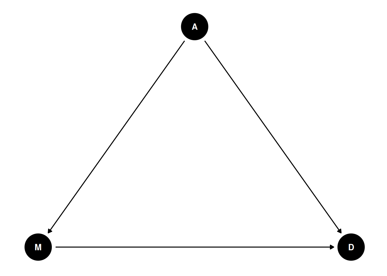

Figure 13.1: DAG for the relationship between marriage rate (M) and divorce rate (D) example, with median age of marriage (A) as a potential confounder.

We can look at how the median age people get married in different states relates to the divorce rate:

ggplot(waffle_divorce,
       aes(x = MedianAgeMarriage, y = Divorce)) +
    geom_point() +
    geom_smooth() +
    labs(x = "Median age marriage (10 years)",
         y = "Divorce rate (per 10 adults)") +
    ggrepel::geom_text_repel(aes(label = Loc))

`geom_smooth()` using method = 'loess' and formula = 'y ~ x'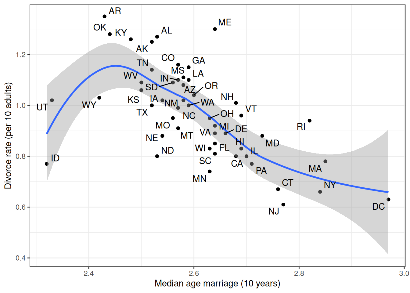

Figure 13.2: Scatter plot of divorce rate (y) vs median age of marriage (x).

13.2.1 Assumptions in a DAG

In a graphical model, there are usually two kinds of assumptions conveyed. Perhaps counterintuitively, the weaker assumptions are the ones you can see, whereas the stronger assumptions are ones you do not see.

For example, a weak assumption is:

• Marriage age may directly influence the number of people who are married

On the other hand, examples of a strong assumption are:

• Marriage rate does not directly influence the age people get married
• there is no other variable in the causal pathway M → D

The last assumption will not hold if there is a common cause of M and D other than A.

13.2.2 Basic Types of Junctions

• Fork: A ← B → C
  • A and C are correlated due to a common cause B
• Chain/Pipe: A → B → C
  • B is on the causal pathway of A to C
• Collider: A → B ← C
  • B is a descendant of both A and C

Going back to our example, there is a fork relation: M → A → D. In this case, A is a confounder when estimating the causal relation between M and D. In this case, the causal effect of M to D can be obtained by adjusting for A, which means looking at the subsets of data where A is constant. In regression, adjustment is obtained by including both M and A as predictors of D.

13.3 The Back-Door Criterion: Estimating Causal Effect in Nonexperimental Data

Randomization is one—but not the only—way to rule out confounding variables. Much progress has been made in clarifying that causal effects can be estimated in nonexperimental data. After all, researchers have not randomly assigned individuals to smoke \(x\) cigarettes per day, but we are confident that smoking causes cancer; we never manipulated the moon’s gravitational force, but we are pretty sure that the moon is a cause of high and low tides.

In a DAG, the back-door criterion can be used to identify variables that we should adjust for to obtain a causal effect. The set of variables to be adjusted should (a) blocks every path between X and Y that contains an arrow entering X and (b) does not contain variables that are descendant of X.

dag4 <- dagitty(
    "dag{
      X -> Y; W1 -> X; U -> W2; W2 -> X; W1 -> Y; U -> Y
    }"
)
latents(dag4) <- "U"
coordinates(dag4) <- list(x = c(X = 0, W1 = 0.66, U = 1.32, W2 = 0.66, Y = 2),
                          y = c(X = 0, W1 = 1, U = 1, W2 = 0.5, Y = 0))
ggdag(dag4) + theme_dag()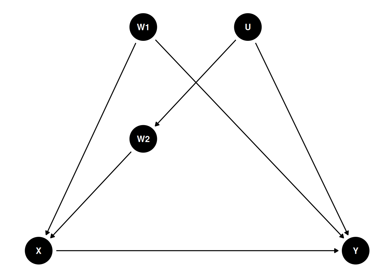

Figure 13.3: DAG for a hypothetical model with two measured and one unobserved confounder.

We can use a function in the daggity package to identify the set of variables that satisfy the back-door criterion. In this case, we say that X and Y are \(d\)-separated by this set of adjusted variables:

adjustmentSets(dag4, exposure = "X", outcome = "Y",
               effect = "direct")

{ W1, W2 }

13.4 Using Multiple Regression Model

\[ \begin{aligned} D_i & \sim N(\mu_i, \sigma) \\ \mu_i & = \beta_0 + \beta_1 A_i + \beta_2 M_i \\ \beta_0 & \sim N(0, 1) \\ \beta_1 & \sim N(0, 1) \\ \beta_2 & \sim N(0, 1) \\ \end{aligned} \]

Assuming a correctly specified DAG, all all assumptions of a linear model are met, \(\beta_2\) is the causal effect of M on D. Here is the brms code:

m1 <- brm(Divorce ~ MedianAgeMarriage + Marriage,
          data = waffle_divorce,
          prior = prior(std_normal(), class = "b") +
              prior(normal(0, 5), class = "Intercept") +
              prior(student_t(4, 0, 3), class = "sigma"),
          seed = 941,
          iter = 4000,
          file = "08_m1"
)

Start sampling

Running MCMC with 4 sequential chains...

Chain 1 Iteration:    1 / 4000 [  0%]  (Warmup) 
Chain 1 Iteration:  100 / 4000 [  2%]  (Warmup) 
Chain 1 Iteration:  200 / 4000 [  5%]  (Warmup) 
Chain 1 Iteration:  300 / 4000 [  7%]  (Warmup) 
Chain 1 Iteration:  400 / 4000 [ 10%]  (Warmup) 
Chain 1 Iteration:  500 / 4000 [ 12%]  (Warmup) 
Chain 1 Iteration:  600 / 4000 [ 15%]  (Warmup) 
Chain 1 Iteration:  700 / 4000 [ 17%]  (Warmup) 
Chain 1 Iteration:  800 / 4000 [ 20%]  (Warmup) 
Chain 1 Iteration:  900 / 4000 [ 22%]  (Warmup) 
Chain 1 Iteration: 1000 / 4000 [ 25%]  (Warmup) 
Chain 1 Iteration: 1100 / 4000 [ 27%]  (Warmup) 
Chain 1 Iteration: 1200 / 4000 [ 30%]  (Warmup) 
Chain 1 Iteration: 1300 / 4000 [ 32%]  (Warmup) 
Chain 1 Iteration: 1400 / 4000 [ 35%]  (Warmup) 
Chain 1 Iteration: 1500 / 4000 [ 37%]  (Warmup) 
Chain 1 Iteration: 1600 / 4000 [ 40%]  (Warmup) 
Chain 1 Iteration: 1700 / 4000 [ 42%]  (Warmup) 
Chain 1 Iteration: 1800 / 4000 [ 45%]  (Warmup) 
Chain 1 Iteration: 1900 / 4000 [ 47%]  (Warmup) 
Chain 1 Iteration: 2000 / 4000 [ 50%]  (Warmup) 
Chain 1 Iteration: 2001 / 4000 [ 50%]  (Sampling) 
Chain 1 Iteration: 2100 / 4000 [ 52%]  (Sampling) 
Chain 1 Iteration: 2200 / 4000 [ 55%]  (Sampling) 
Chain 1 Iteration: 2300 / 4000 [ 57%]  (Sampling) 
Chain 1 Iteration: 2400 / 4000 [ 60%]  (Sampling) 
Chain 1 Iteration: 2500 / 4000 [ 62%]  (Sampling) 
Chain 1 Iteration: 2600 / 4000 [ 65%]  (Sampling) 
Chain 1 Iteration: 2700 / 4000 [ 67%]  (Sampling) 
Chain 1 Iteration: 2800 / 4000 [ 70%]  (Sampling) 
Chain 1 Iteration: 2900 / 4000 [ 72%]  (Sampling) 
Chain 1 Iteration: 3000 / 4000 [ 75%]  (Sampling) 
Chain 1 Iteration: 3100 / 4000 [ 77%]  (Sampling) 
Chain 1 Iteration: 3200 / 4000 [ 80%]  (Sampling) 
Chain 1 Iteration: 3300 / 4000 [ 82%]  (Sampling) 
Chain 1 Iteration: 3400 / 4000 [ 85%]  (Sampling) 
Chain 1 Iteration: 3500 / 4000 [ 87%]  (Sampling) 
Chain 1 Iteration: 3600 / 4000 [ 90%]  (Sampling) 
Chain 1 Iteration: 3700 / 4000 [ 92%]  (Sampling) 
Chain 1 Iteration: 3800 / 4000 [ 95%]  (Sampling) 
Chain 1 Iteration: 3900 / 4000 [ 97%]  (Sampling) 
Chain 1 Iteration: 4000 / 4000 [100%]  (Sampling) 
Chain 1 finished in 0.0 seconds.
Chain 2 Iteration:    1 / 4000 [  0%]  (Warmup) 
Chain 2 Iteration:  100 / 4000 [  2%]  (Warmup) 
Chain 2 Iteration:  200 / 4000 [  5%]  (Warmup) 
Chain 2 Iteration:  300 / 4000 [  7%]  (Warmup) 
Chain 2 Iteration:  400 / 4000 [ 10%]  (Warmup) 
Chain 2 Iteration:  500 / 4000 [ 12%]  (Warmup) 
Chain 2 Iteration:  600 / 4000 [ 15%]  (Warmup) 
Chain 2 Iteration:  700 / 4000 [ 17%]  (Warmup) 
Chain 2 Iteration:  800 / 4000 [ 20%]  (Warmup) 
Chain 2 Iteration:  900 / 4000 [ 22%]  (Warmup) 
Chain 2 Iteration: 1000 / 4000 [ 25%]  (Warmup) 
Chain 2 Iteration: 1100 / 4000 [ 27%]  (Warmup) 
Chain 2 Iteration: 1200 / 4000 [ 30%]  (Warmup) 
Chain 2 Iteration: 1300 / 4000 [ 32%]  (Warmup) 
Chain 2 Iteration: 1400 / 4000 [ 35%]  (Warmup) 
Chain 2 Iteration: 1500 / 4000 [ 37%]  (Warmup) 
Chain 2 Iteration: 1600 / 4000 [ 40%]  (Warmup) 
Chain 2 Iteration: 1700 / 4000 [ 42%]  (Warmup) 
Chain 2 Iteration: 1800 / 4000 [ 45%]  (Warmup) 
Chain 2 Iteration: 1900 / 4000 [ 47%]  (Warmup) 
Chain 2 Iteration: 2000 / 4000 [ 50%]  (Warmup) 
Chain 2 Iteration: 2001 / 4000 [ 50%]  (Sampling) 
Chain 2 Iteration: 2100 / 4000 [ 52%]  (Sampling) 
Chain 2 Iteration: 2200 / 4000 [ 55%]  (Sampling) 
Chain 2 Iteration: 2300 / 4000 [ 57%]  (Sampling) 
Chain 2 Iteration: 2400 / 4000 [ 60%]  (Sampling) 
Chain 2 Iteration: 2500 / 4000 [ 62%]  (Sampling) 
Chain 2 Iteration: 2600 / 4000 [ 65%]  (Sampling) 
Chain 2 Iteration: 2700 / 4000 [ 67%]  (Sampling) 
Chain 2 Iteration: 2800 / 4000 [ 70%]  (Sampling) 
Chain 2 Iteration: 2900 / 4000 [ 72%]  (Sampling) 
Chain 2 Iteration: 3000 / 4000 [ 75%]  (Sampling) 
Chain 2 Iteration: 3100 / 4000 [ 77%]  (Sampling) 
Chain 2 Iteration: 3200 / 4000 [ 80%]  (Sampling) 
Chain 2 Iteration: 3300 / 4000 [ 82%]  (Sampling) 
Chain 2 Iteration: 3400 / 4000 [ 85%]  (Sampling) 
Chain 2 Iteration: 3500 / 4000 [ 87%]  (Sampling) 
Chain 2 Iteration: 3600 / 4000 [ 90%]  (Sampling) 
Chain 2 Iteration: 3700 / 4000 [ 92%]  (Sampling) 
Chain 2 Iteration: 3800 / 4000 [ 95%]  (Sampling) 
Chain 2 Iteration: 3900 / 4000 [ 97%]  (Sampling) 
Chain 2 Iteration: 4000 / 4000 [100%]  (Sampling) 
Chain 2 finished in 0.0 seconds.
Chain 3 Iteration:    1 / 4000 [  0%]  (Warmup) 
Chain 3 Iteration:  100 / 4000 [  2%]  (Warmup) 
Chain 3 Iteration:  200 / 4000 [  5%]  (Warmup) 
Chain 3 Iteration:  300 / 4000 [  7%]  (Warmup) 
Chain 3 Iteration:  400 / 4000 [ 10%]  (Warmup) 
Chain 3 Iteration:  500 / 4000 [ 12%]  (Warmup) 
Chain 3 Iteration:  600 / 4000 [ 15%]  (Warmup) 
Chain 3 Iteration:  700 / 4000 [ 17%]  (Warmup) 
Chain 3 Iteration:  800 / 4000 [ 20%]  (Warmup) 
Chain 3 Iteration:  900 / 4000 [ 22%]  (Warmup) 
Chain 3 Iteration: 1000 / 4000 [ 25%]  (Warmup) 
Chain 3 Iteration: 1100 / 4000 [ 27%]  (Warmup) 
Chain 3 Iteration: 1200 / 4000 [ 30%]  (Warmup) 
Chain 3 Iteration: 1300 / 4000 [ 32%]  (Warmup) 
Chain 3 Iteration: 1400 / 4000 [ 35%]  (Warmup) 
Chain 3 Iteration: 1500 / 4000 [ 37%]  (Warmup) 
Chain 3 Iteration: 1600 / 4000 [ 40%]  (Warmup) 
Chain 3 Iteration: 1700 / 4000 [ 42%]  (Warmup) 
Chain 3 Iteration: 1800 / 4000 [ 45%]  (Warmup) 
Chain 3 Iteration: 1900 / 4000 [ 47%]  (Warmup) 
Chain 3 Iteration: 2000 / 4000 [ 50%]  (Warmup) 
Chain 3 Iteration: 2001 / 4000 [ 50%]  (Sampling) 
Chain 3 Iteration: 2100 / 4000 [ 52%]  (Sampling) 
Chain 3 Iteration: 2200 / 4000 [ 55%]  (Sampling) 
Chain 3 Iteration: 2300 / 4000 [ 57%]  (Sampling) 
Chain 3 Iteration: 2400 / 4000 [ 60%]  (Sampling) 
Chain 3 Iteration: 2500 / 4000 [ 62%]  (Sampling) 
Chain 3 Iteration: 2600 / 4000 [ 65%]  (Sampling) 
Chain 3 Iteration: 2700 / 4000 [ 67%]  (Sampling) 
Chain 3 Iteration: 2800 / 4000 [ 70%]  (Sampling) 
Chain 3 Iteration: 2900 / 4000 [ 72%]  (Sampling) 
Chain 3 Iteration: 3000 / 4000 [ 75%]  (Sampling) 
Chain 3 Iteration: 3100 / 4000 [ 77%]  (Sampling) 
Chain 3 Iteration: 3200 / 4000 [ 80%]  (Sampling) 
Chain 3 Iteration: 3300 / 4000 [ 82%]  (Sampling) 
Chain 3 Iteration: 3400 / 4000 [ 85%]  (Sampling) 
Chain 3 Iteration: 3500 / 4000 [ 87%]  (Sampling) 
Chain 3 Iteration: 3600 / 4000 [ 90%]  (Sampling) 
Chain 3 Iteration: 3700 / 4000 [ 92%]  (Sampling) 
Chain 3 Iteration: 3800 / 4000 [ 95%]  (Sampling) 
Chain 3 Iteration: 3900 / 4000 [ 97%]  (Sampling) 
Chain 3 Iteration: 4000 / 4000 [100%]  (Sampling) 
Chain 3 finished in 0.1 seconds.
Chain 4 Iteration:    1 / 4000 [  0%]  (Warmup) 
Chain 4 Iteration:  100 / 4000 [  2%]  (Warmup) 
Chain 4 Iteration:  200 / 4000 [  5%]  (Warmup) 
Chain 4 Iteration:  300 / 4000 [  7%]  (Warmup) 
Chain 4 Iteration:  400 / 4000 [ 10%]  (Warmup) 
Chain 4 Iteration:  500 / 4000 [ 12%]  (Warmup) 
Chain 4 Iteration:  600 / 4000 [ 15%]  (Warmup) 
Chain 4 Iteration:  700 / 4000 [ 17%]  (Warmup) 
Chain 4 Iteration:  800 / 4000 [ 20%]  (Warmup) 
Chain 4 Iteration:  900 / 4000 [ 22%]  (Warmup) 
Chain 4 Iteration: 1000 / 4000 [ 25%]  (Warmup) 
Chain 4 Iteration: 1100 / 4000 [ 27%]  (Warmup) 
Chain 4 Iteration: 1200 / 4000 [ 30%]  (Warmup) 
Chain 4 Iteration: 1300 / 4000 [ 32%]  (Warmup) 
Chain 4 Iteration: 1400 / 4000 [ 35%]  (Warmup) 
Chain 4 Iteration: 1500 / 4000 [ 37%]  (Warmup) 
Chain 4 Iteration: 1600 / 4000 [ 40%]  (Warmup) 
Chain 4 Iteration: 1700 / 4000 [ 42%]  (Warmup) 
Chain 4 Iteration: 1800 / 4000 [ 45%]  (Warmup) 
Chain 4 Iteration: 1900 / 4000 [ 47%]  (Warmup) 
Chain 4 Iteration: 2000 / 4000 [ 50%]  (Warmup) 
Chain 4 Iteration: 2001 / 4000 [ 50%]  (Sampling) 
Chain 4 Iteration: 2100 / 4000 [ 52%]  (Sampling) 
Chain 4 Iteration: 2200 / 4000 [ 55%]  (Sampling) 
Chain 4 Iteration: 2300 / 4000 [ 57%]  (Sampling) 
Chain 4 Iteration: 2400 / 4000 [ 60%]  (Sampling) 
Chain 4 Iteration: 2500 / 4000 [ 62%]  (Sampling) 
Chain 4 Iteration: 2600 / 4000 [ 65%]  (Sampling) 
Chain 4 Iteration: 2700 / 4000 [ 67%]  (Sampling) 
Chain 4 Iteration: 2800 / 4000 [ 70%]  (Sampling) 
Chain 4 Iteration: 2900 / 4000 [ 72%]  (Sampling) 
Chain 4 Iteration: 3000 / 4000 [ 75%]  (Sampling) 
Chain 4 Iteration: 3100 / 4000 [ 77%]  (Sampling) 
Chain 4 Iteration: 3200 / 4000 [ 80%]  (Sampling) 
Chain 4 Iteration: 3300 / 4000 [ 82%]  (Sampling) 
Chain 4 Iteration: 3400 / 4000 [ 85%]  (Sampling) 
Chain 4 Iteration: 3500 / 4000 [ 87%]  (Sampling) 
Chain 4 Iteration: 3600 / 4000 [ 90%]  (Sampling) 
Chain 4 Iteration: 3700 / 4000 [ 92%]  (Sampling) 
Chain 4 Iteration: 3800 / 4000 [ 95%]  (Sampling) 
Chain 4 Iteration: 3900 / 4000 [ 97%]  (Sampling) 
Chain 4 Iteration: 4000 / 4000 [100%]  (Sampling) 
Chain 4 finished in 0.0 seconds.

All 4 chains finished successfully.
Mean chain execution time: 0.0 seconds.
Total execution time: 0.6 seconds.

Loading required package: rstan

Loading required package: StanHeaders

rstan version 2.32.5 (Stan version 2.32.2)

For execution on a local, multicore CPU with excess RAM we recommend calling
options(mc.cores = parallel::detectCores()).
To avoid recompilation of unchanged Stan programs, we recommend calling
rstan_options(auto_write = TRUE)
For within-chain threading using `reduce_sum()` or `map_rect()` Stan functions,
change `threads_per_chain` option:
rstan_options(threads_per_chain = 1)

Attaching package: 'rstan'

The following object is masked from 'package:tidyr':

    extract

13.4.1 Table

msummary(m1,
         estimate = "{estimate} [{conf.low}, {conf.high}]",
         statistic = NULL, fmt = 2
)

Warning: 
`modelsummary` uses the `performance` package to extract goodness-of-fit
statistics from models of this class. You can specify the statistics you wish
to compute by supplying a `metrics` argument to `modelsummary`, which will then
push it forward to `performance`. Acceptable values are: "all", "common",
"none", or a character vector of metrics names. For example: `modelsummary(mod,
metrics = c("RMSE", "R2")` Note that some metrics are computationally
expensive. See `?performance::performance` for details.
 This warning appears once per session.

Table 13.1: Model results for the divorce rate example.

	(1)
b_Intercept	3.49 [1.98, 5.02]
b_MedianAgeMarriage	−0.93 [−1.43, −0.45]
b_Marriage	−0.04 [−0.20, 0.12]
sigma	0.15 [0.12, 0.19]
Num.Obs.	50
R2	0.349
R2 Adj.	0.283
ELPD	21.0
ELPD s.e.	6.4
LOOIC	−42.0
LOOIC s.e.	12.9
WAIC	−42.2
RMSE	0.14

As shown in the table, when holding constant the median marriage age of states, marriage rate has only a small effect on divorce rate.

13.4.2 Posterior predictive checks

pp_check(m1, ndraws = 100) # density
pp_check(m1, type = "intervals", x = "Marriage") +
    labs(x = "Marriage", y = "Divorce")

Using all posterior draws for ppc type 'intervals' by default.

pp_check(m1, type = "intervals", x = "MedianAgeMarriage") +
    labs(x = "MedianAgeMarriage", y = "Divorce")

Using all posterior draws for ppc type 'intervals' by default.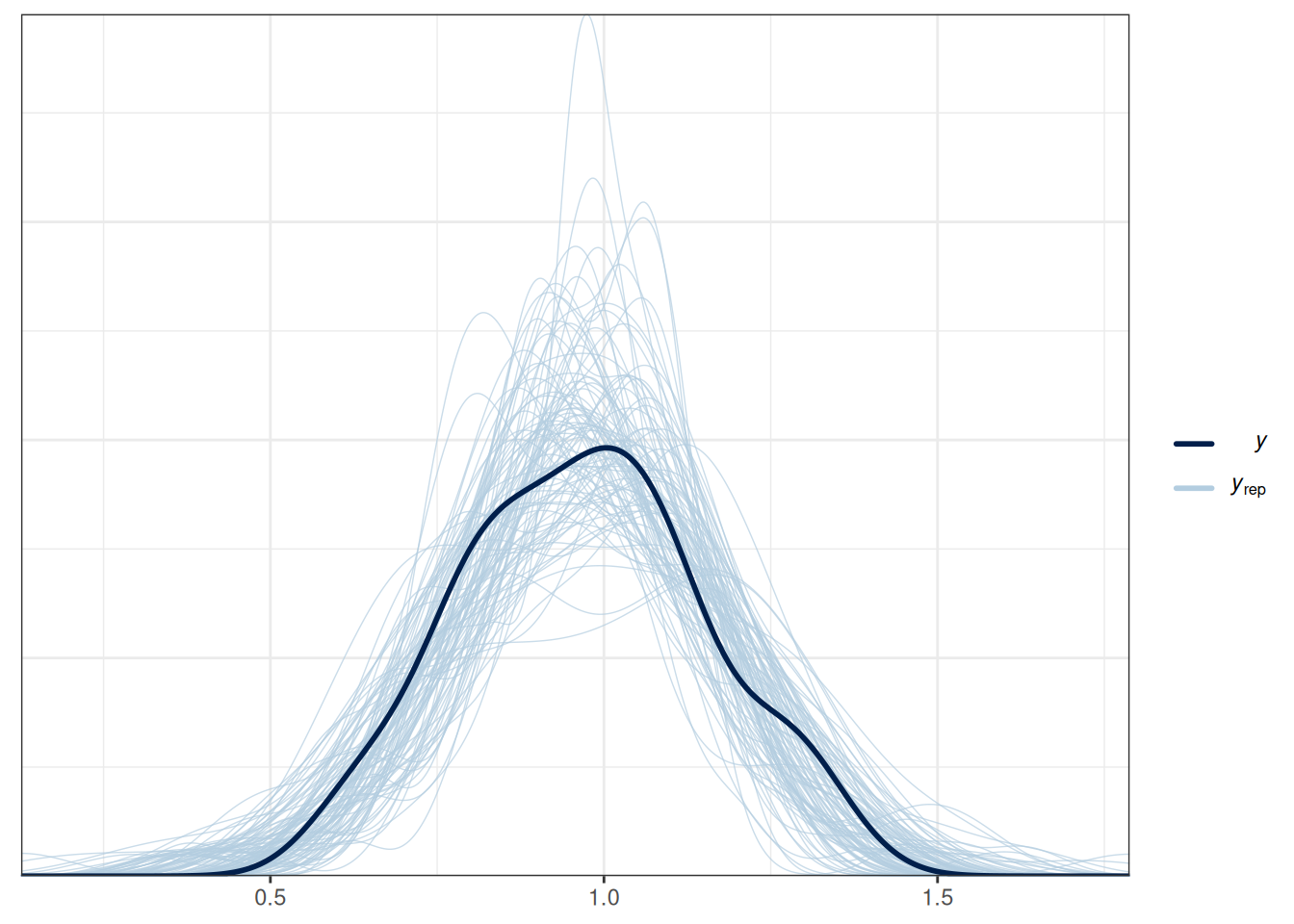

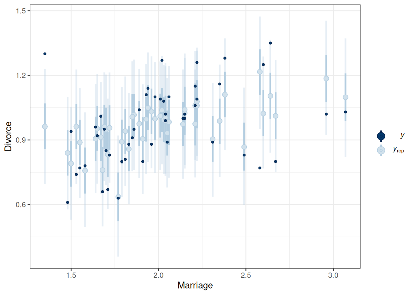
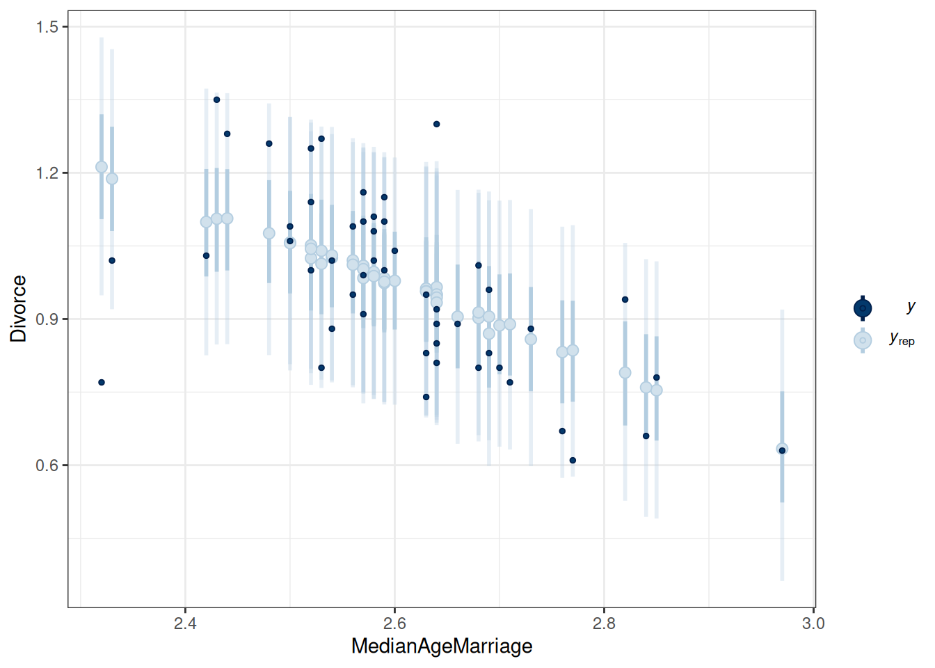
(a) Posterior predictive density of divorce rate.

(b) Posterior predictive intervals of marriage rate predicting divorce rate.

(c) Posterior predictive intervals of median marriage age predicting marriage rate.

Figure 13.4: Posterior predictive checks for the multiple regression model.

The model does not fit every state (e.g., UT, ME, ID).

13.5 Predicting an Intervention

If the causal assumption in our DAG is reasonable, we have obtained an estimate of the causal effect of marriage rate on divorce rate at the state level. This allows us to answer questions like

What would happen to the divorce rate if we encouraged more people to get married (so the marriage rate would increase by 10 percentage points)?

We can use the Bayesian model, which is generative, to make such predictions. Consider a state with a marriage rate of 2 (per 10 adults). The predicted divorce rate is

\[ \beta_0 + \beta_1 A + \beta_2 (2) \]

Consider an intervention that increases the marriage rate from 2 to 3. The predicted divorce rate will be

\[ \beta_0 + \beta_1 A + \beta_2 (3) \]

The change in divorce rate is

\[ \beta_0 + \beta_1 A + \beta_2 (3) - \beta_0 + \beta_1 A + \beta_2 (2) = \beta_2 \]

Here is what the model would predict in terms of the change in the divorce rate (holding median marriage age to 25 years old), using R:

pred_df <- data.frame(
    Marriage = c(2, 3),
    MedianAgeMarriage = c(2.5, 2.5)
)
cbind(pred_df, fitted(m1, newdata = pred_df)) %>%
    knitr::kable(digits = 3)

Marriage	MedianAgeMarriage	Estimate	Est.Error	Q2.5	Q97.5
2	2.5	1.068	0.035	1.002	1.138
3	2.5	1.026	0.067	0.894	1.160

The difference should be just the estimate of \(\beta_2\), which has the following posterior distribution:

mcmc_dens(m1, pars = "b_Marriage")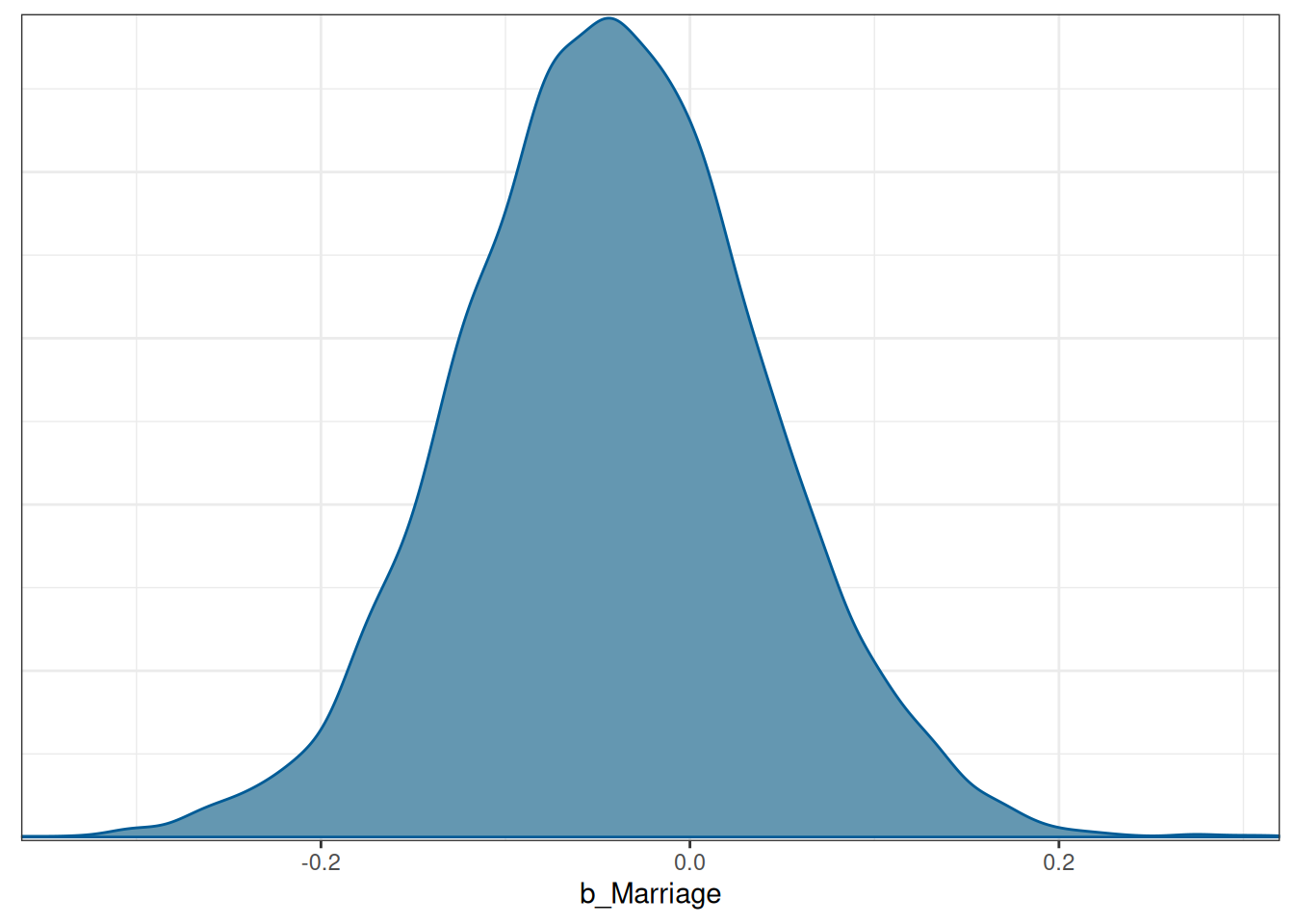

Figure 13.5: Estimated “causal” effect of marriage rate on divorce rate, based on the specified DAG and a linear model.

13.6 Collider

A collider is a descendant of two parent nodes. When one holds the collider constant, it induces a spurious association between the parents. This leads to many unexpected results in data analysis and daily life. For example, consider people who are nice and who are good-looking. Is there an association between a person being nice and a person being good-looking? Maybe. But this association can be induced when we condition on a collider. Let’s say a friend of yours only dates people who are either nice or good-looking. So we have this colliding relation:

Nice → Dating ← Good looking

Suppose you look at just the people that your friend dated. In that case, they are either nice or good-looking, but the fact that you select to look at (condition on) only the people that your friend dated would automatically eliminate people who are neither nice nor good-looking. This induces a spurious negative association between nice and good-looking, so your friend may believe that nice people would be less likely to have appearances that fit their taste, and vice versa.

As another example, is research that is newsworthy less trustworthy? There could be a negative association due to collider bias, because people who select research to be reported, funded, or published, consider both newsworthiness and trustworthiness. Assume that trustworthiness has no causal relation with newsworthiness, below shows what happens when we only focus on papers that are either high on newsworthiness or trustworthiness:

set.seed(2221) # different seed from the text
num_proposals <- 200 # number of grant proposals
prop_selected <- 0.1 # proportion to select
# Simulate independent newsworthiness and trustworthiness
plot_dat <- data.frame(
    nw = rnorm(num_proposals),
    tw = rnorm(num_proposals)
)
plot_dat <- plot_dat |>
    mutate(total = nw + tw)
sel_dat <- plot_dat |>
    # select top 10% of combined scores
    slice_max(order_by = total, prop = prop_selected)
plot_dat |>
    ggplot(aes(x = nw, y = tw)) +
    geom_point() +
    geom_point(data = sel_dat, shape = 1, size = 3,
               color = "red") +
    geom_smooth(method = "lm", se = FALSE) +
    geom_smooth(data = sel_dat, method = "lm", se = FALSE,
                col = "purple") +
    labs(x = "newsworthiness", y = "trustworthiness")

`geom_smooth()` using formula = 'y ~ x'
`geom_smooth()` using formula = 'y ~ x'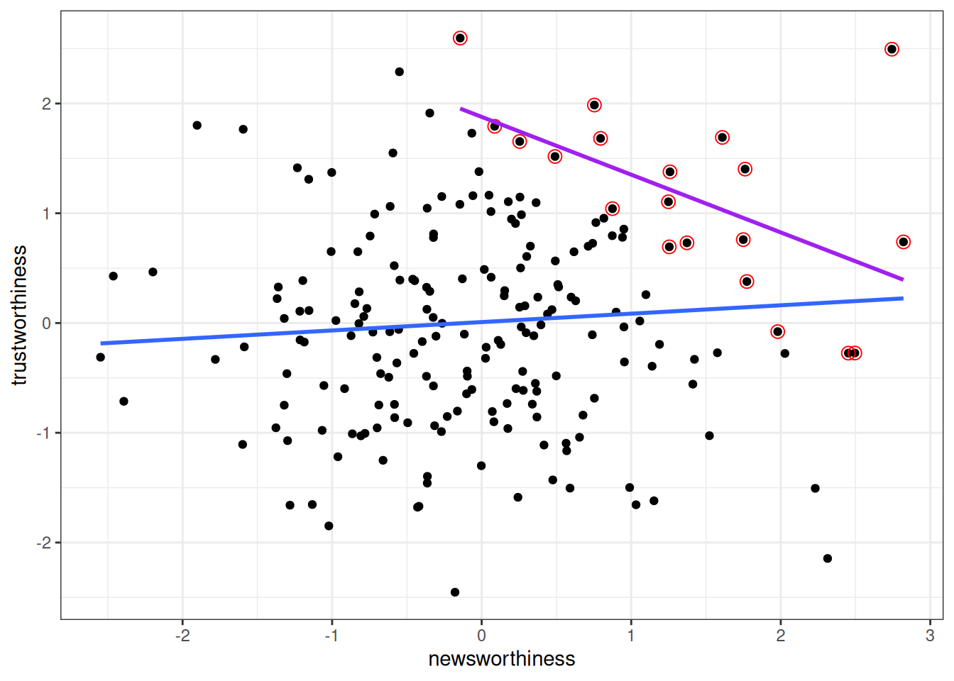

Figure 13.6: Simulation of newsworthiness and trustworthiness.

As you can see, a negative correlation happens. This is collider bias: spurious correlation due to conditioning on the common descendant. This also goes by the name Berkson’s Paradox.

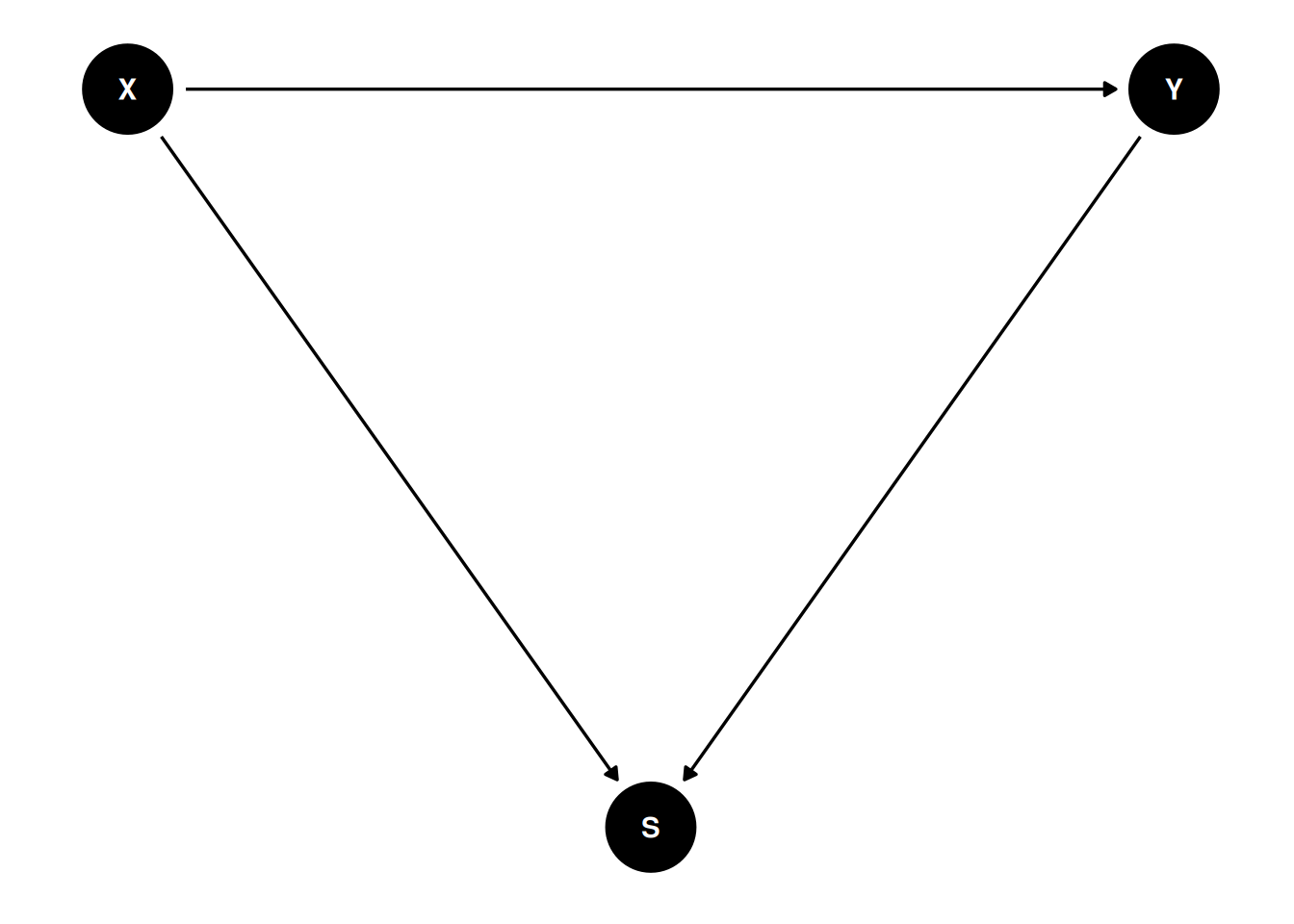
In the DAG below, X and Y have no causal association. Conditioning on S, however, induces a negative correlation between X and Y. With the DAG below,

Generally speaking, do not condition on a collider, unless you’re going to de-confound the spurious association using other variables.

dag7 <- dagitty(
    "dag{
      X -> Y; X -> S; Y -> S
    }"
)
coordinates(dag7) <- list(x = c(X = 0, S = 1, Y = 2),
                          y = c(X = 0, S = -1, Y = 0))
ggdag(dag7) + theme_dag()

Figure 13.7: DAG with collider bias.

Age and Happiness, conditioned on Marital Status (Example from text)

In this example, we assume that age and happiness are not related, but as people age, they are more likely to get married.

# Code adapted from the rethinking package (https://github.com/rmcelreath/rethinking/blob/master/R/sim_happiness.R)
sim_happiness <- function(seed = 1977, N_years = 100,
                          max_age = 65, N_births = 50,
                          aom = 18) {
    set.seed(seed)
    H <- M <- A <- c()
    for (t in seq_len(N_years)) {
        A <- A + 1 # age existing individuals
        A <- c(A, rep(1, N_births)) # newborns
        H <- c(H, seq(from = 1, to = 5, length.out = N_births)) # sim happiness trait - never changes
        M <- c(M, rep(0, N_births)) # not yet married
        # for each person over 17, chance get married
        M[A >= aom & M == 0] <- 
            rbinom(A[A >= aom & M == 0], size = 1,
                   prob = plogis(H[A >= aom & M == 0] - 7.9))
        # mortality
        deaths <- which(A > max_age)
        if (length(deaths) > 0) {
            A <- A[-deaths]
            H <- H[-deaths]
            M <- M[-deaths]
        }
    }
    d <- data.frame(age = A, married = M, happiness = H)
    return(d)
}
dd <- sim_happiness(2024, N_years = 100)

ggplot(dd, aes(x = age, y = happiness)) +
    geom_point(alpha = .1, size = .5)

Figure 13.8: Age and happiness.

ggplot(dd[dd$married == 1, ], aes(x = age, y = happiness)) +
    geom_point(alpha = .5, size = .5)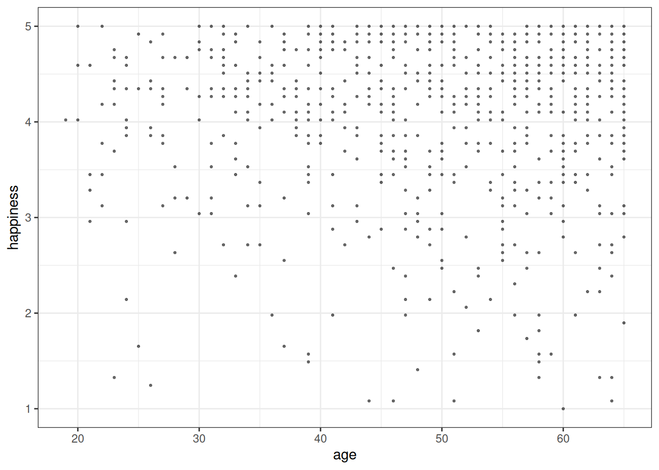

Figure 13.9: Age and happiness, conditioned on married couples.

Some other collider examples:

• impulsivity → high-risk youth ← delinquency
• healthcare worker → COVID-19 testing ← COVID-19 severity
• standardized test → admission ← research skills
• maternal smoking → birth weight → birth defect ← mortality

13.7 Some Additional References

• https://doi.org/10.1177/25152459221095823
• https://doi.org/10.1038/s41562-024-01939-z

McElreath, R. (2020). Statistical rethinking: a Bayesian course with examples in R and Stan (Second edition). CRC Press.

---

1. See this paper: https://doi.org/10.1177/1745691620921521 for an argument of how the taboo against causal inference has impeded the progress of psychology research.