3 Bayes’s Theorem

The Bayes’s theorem is, surprisingly (or unsurprisingly), very simple:

\[ P(B \mid A) = \frac{P(A \mid B) P(B)}{P(A)} \]

More generally, we can expand it to incorporate the law of total probability to make it more applicable to data analysis. Consider $B_i$ as one of the $n$ many possible mutually exclusive events, then \[ \begin{aligned} P(B_i \mid A) & = \frac{P(A \mid B_i) P(B_i)}{P(A)} \\ & = \frac{P(A \mid B_i) P(B_i)} {P(A \mid B_1)P(B_1) + P(A \mid B_2)P(B_2) + \cdots + P(A \mid B_n)P(B_n)} \\ & = \frac{P(A \mid B_i) P(B_i)}{\sum_{k = 1}^n P(A \mid B_k)P(B_k)} \end{aligned} \]

If $B_i$ is a continuous variable, we will replace the sum by an integral, \[ P(B_i \mid A) = \frac{P(A \mid B_i) P(B_i)}{\int_k P(A \mid B_k)P(B_k)} \] The denominator is not important for practical Bayesian analysis, therefore, it is sufficient to write the above equality as

\[ P(B_i \mid A) \propto P(A \mid B_i) P(B_i) \]

3.1 Example 1: Base rate fallacy (From Wikipedia)

Question
Solution

A police officer stops a driver at random and does a breathalyzer test for the driver. The breathalyzer is known to detect true drunkenness 100% of the time, but in 1% of the cases, it gives a false positive when the driver is sober. We also know that, in general, for every 1,000 drivers passing through that spot, one is driving drunk. Suppose that the breathalyzer shows positive for the driver. What is the probability that the driver is truly drunk?

$P(\text{positive} | \text{drunk}) = 1$
$P(\text{positive} | \text{sober}) = 0.01$
$P(\text{drunk}) = 1 / 1000$
$P(\text{sober}) = 999 / 1000$

Using Bayes’ Theorem,

\[ \begin{aligned} P(\text{drunk} | \text{positive}) & = \frac{P(\text{positive} | \text{drunk}) P(\text{drunk})} {P(\text{positive} | \text{drunk}) P(\text{drunk}) + P(\text{positive} | \text{sober}) P(\text{sober})} \\ & = \frac{1 \times 0.001}{1 \times 0.001 + 0.01 \times 0.999} \\ & = 100 / 1099 \approx 0.091 \end{aligned} \]

So there is less than a 10% chance that the driver is drunk even when the breathalyzer shows positive.

You can verify that with a simulation using R:

set.seed(4)
truly_drunk <- c(rep("drunk", 100), rep("sober", 100 * 999))
table(truly_drunk)

#> truly_drunk
#> drunk sober 
#>   100 99900

breathalyzer_test <- ifelse(truly_drunk == "drunk",
    # If drunk, 100% chance of showing positive
    "positive",
    # If not drunk, 1% chance of showing positive
    sample(c("positive", "negative"), 999000,
        replace = TRUE, prob = c(.01, .99)
    )
)
# Check the probability p(positive | sober)
table(breathalyzer_test[truly_drunk == "sober"])

#> 
#> negative positive 
#>    98903      997

# 997 / 99900 = 0.00997998, so the error rate is less than 1%
# Now, Check the probability p(drunk | positive)
table(truly_drunk[breathalyzer_test == "positive"])

#> 
#> drunk sober 
#>   100   997

# 100 / (100 + 997) = 0.0911577, which is only 9.1%!

3.2 Bayesian Statistics

Bayesian statistics is a way to estimate some parameter $\theta$ (i.e., some quantities of interest, such as the population mean, regression coefficient, etc) by applying Bayes’ Theorem.

\[ P(\theta | D) \propto P(D | \theta) P(\theta) \]

There are three components in the above equality:

$P(D | \theta)$, the probability that you observe data $D$, given the parameter $\theta$; this is called the likelihood (Note: It is the likelihood of $\theta$, but probability about $y$)
$P(\theta)$, the probability distribution $\theta$, without referring to the data $D$. This usually requires appeals to one’s degree of belief, and so is called the prior
$P(\theta | y)$, the updated probability distribution of $\theta$, after observing the data $D$; this is called the posterior

On the other hand, classical/frequentist statistics focuses solely on the likelihood function.¹ In Bayesian statistics, the goal is to update one’s belief about $\theta$ based on the observed data $D$.

3.3 Example 2: Locating a Plane

Consider a highly simplified scenario of locating a missing plane in the sea. Assume that we know the plane, before missing, happened to be flying at the same latitude, heading west across the Pacific, so we only need to find its longitude. We want to go out to collect debris (data) so that we can narrow the location ($\theta$) of the plane down.

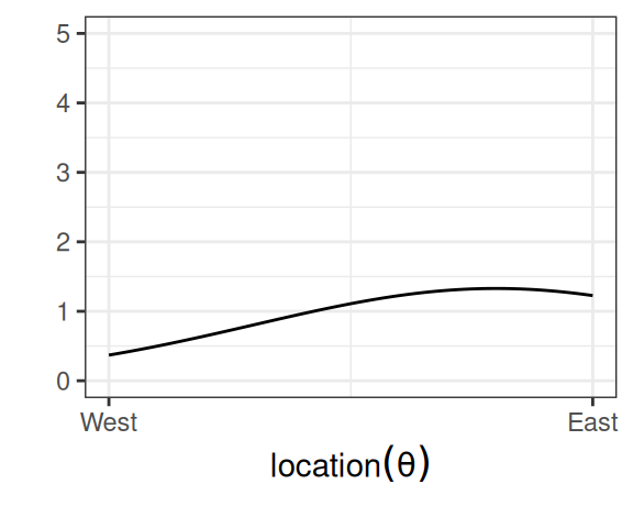
We start with our prior. Assume that we have some rough idea where the plane should be, so we express our belief in a probability distribution like the following:

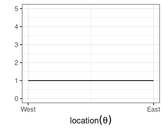
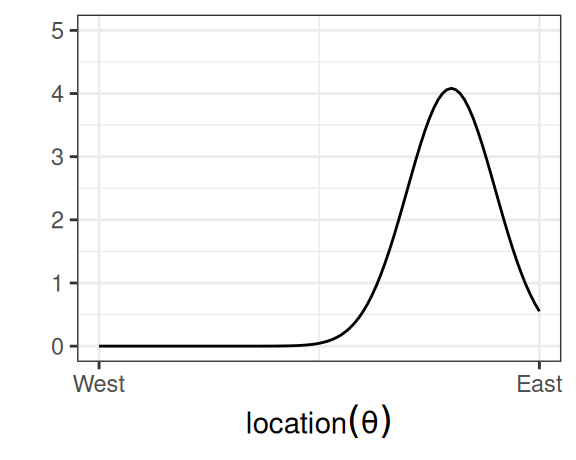
which says that our belief is that the plane is about twice more likely to be towards the east than towards the west. Below are two other options for priors (out of infinitely many), one providing virtually no information and the other encoding stronger information:

The prior is chosen to reflect the researcher’s belief, so different researchers will likely formulate a different prior for the same problem, and that’s okay as long as the prior is reasonable and justified. Later, we will learn that in regular Bayesian analyses, with a moderate sample size, different priors generally only make negligible differences.

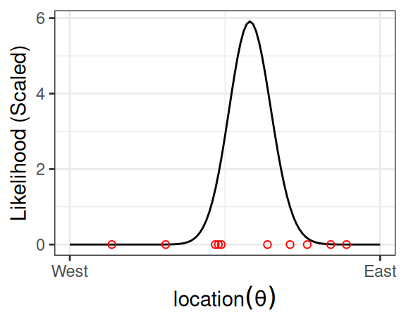
Now, assume that we have collected debris in the locations shown in the graph,

Now, from Bayes’s Theorem,

\[ \text{Posterior Probability} \propto \text{Prior Probability} \times \text{Likelihood} \]

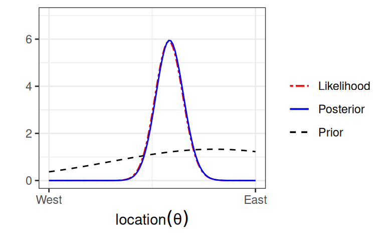
So we can simply multiply the prior probabilities and the likelihood to get the posterior probability for every location. A rescaling step is needed to ensure that the area under the curve will be 1, which is usually performed by the software.

As illustrated below, the posterior distribution is a synthesis of (a) the prior and (b) the data (likelihood).

Influence of Prior
Influence of More Data

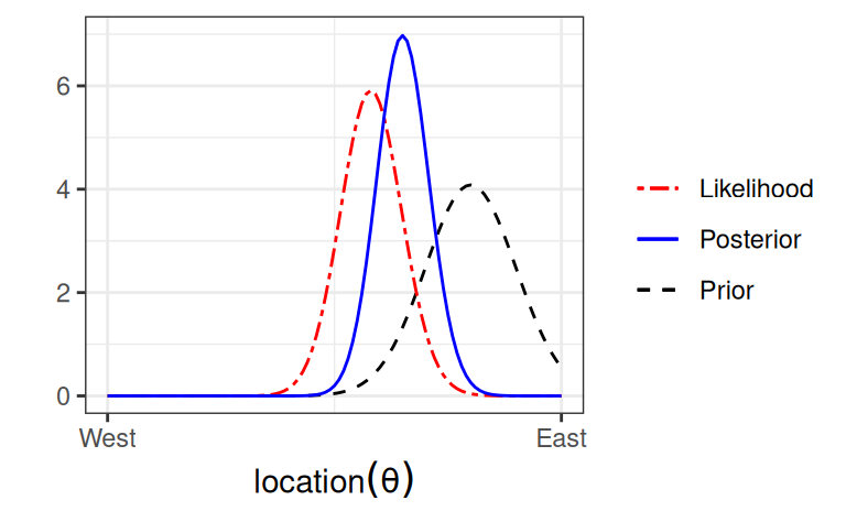
Figure 3.5 shows what happen with a stronger prior:

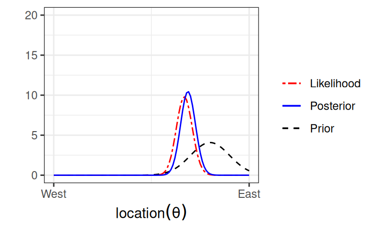
Figure 3.6 shows what happen with 20 more data points:

3.4 Data-Order Invariance

In many data analysis applications, researchers collect some data $D_1$, and then collect some more data $D_2$. An example would be researchers conducting two separate experiments to study the same research question. In Bayesian statistics, one can consider three ways to obtain the posterior:

Update the belief with $D_1$, and then with $D_2$
Update the belief with $D_2$, and then with $D_1$
Update the belief with both $D_1$ and $D_2$ simultaneously

Whether these three ways give the same posterior depends on whether data-order invariance holds. If the inference of $D_1$ does not depend on $D_2$, or vice versa, then all three ways lead to the same posterior. Specifically, if we have conditional independence such that \[ P(D_1, D_2 \mid \theta) = P(D_1 \mid \theta) P(D_2 \mid \theta), \] then one can show all three ways give the same posterior (see section 4.4 and 4.5 of Johnson et al., 2022).

Exchangeability*

Exchangeability is an important concept in Bayesian statistics. Data are exchangeable when the joint distribution, $P(D_1, \ldots, D_N)$, does not depend on the ordering of the data. A simple way to think about it is if you scramble the order of your outcome variable in your data set and still can obtain the same statistical results, then the data are exchangeable. An example situation where data are not exchangeable is

$D_1$ is from year 1990, $D_2$ is from year 2020, and the parameter $\theta$ changes from 1990 to 2020

When data are exchangeable, conditional independence would generally hold.²

3.5 Bernoulli Likelihood

For binary data $y$ (e.g., coin flip, pass/fail, diagnosed/not), an intuitive way to analyze is to use a Bernoulli model: \[ \begin{aligned} P(y = 1 \mid \theta) = \theta \\ P(y = 0 \mid \theta) = 1 - \theta \end{aligned}, \] which is more compactly written as \[ P(y \mid \theta) = \theta^y (1 - \theta)^{(1 - y)}, \] where $\theta \in [0, 1]$ is the probability of a “1”. You can verify that the compact form is the same as the longer form.

3.5.1 Multiple Observations

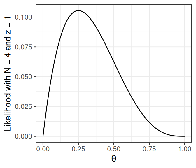
When there are more than one $y$, say $y_1, \ldots, y_N$, that are conditionally independent, we have \[ \begin{aligned} P(y_1, \ldots, y_N \mid \theta) & = \prod_{i = 1}^N P(y_i \mid \theta) \\ & = \theta^{\sum_{i = 1}^N y_i} (1 - \theta)^{\sum_{i = 1}^N (1 - y_i)} \\ & = \theta^z (1 - \theta)^{N - z} \end{aligned}, \] where $z$ is the number of “1”s (e.g., the number of heads in coin flips). Note that the likelihood only depends on $z$, not the individual $y$s. In other words, the likelihood is the same as long as there are $z$ heads, regardless of when those heads occur.

Let’s say $N$ = 4 and $z$ = 1. We can plot the likelihood in R:

# Write the likelihood as a function of theta
lik <- function(th, num_flips = 4, num_heads = 1) {
    th ^ num_heads * (1 - th) ^ (num_flips - num_heads)
}
# Likelihood of theta = 0.5
lik(0.5)

#> [1] 0.0625

# Plot the likelihood
ggplot(data.frame(th = c(0, 1)), aes(x = th)) +
    # `stat_function` for plotting a function
    stat_function(fun = lik) +
    # use `expression()` to get greek letters
    labs(x = expression(theta),
    y = "Likelihood with N = 4 and z = 1")

Figure 3.7: Binomial likelihood function with $N$ = 4 and $z$ = 1

3.5.2 Setting Priors

Remember again the relationship between the prior and the posterior: \[P(\theta | y) \propto P(y | \theta) P(\theta)\] The posterior distributions are mathematically determined once the priors and the likelihood are set. However, the mathematical form of the posterior is sometimes very difficult to deal with.

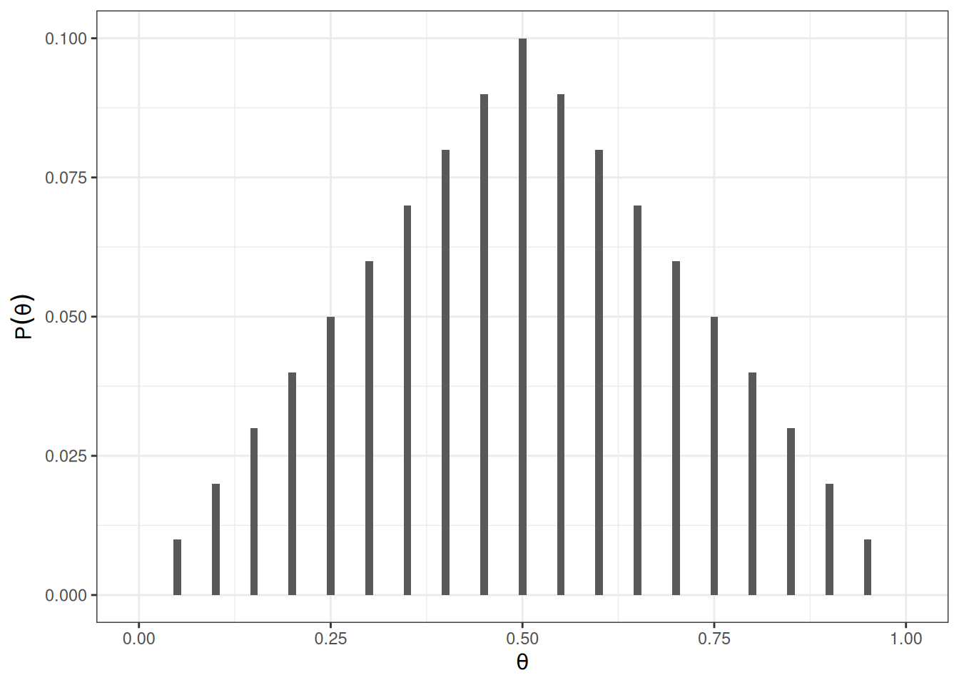
One straightforward, brute-force method is to discretize the parameter space into a number of points. For example, by taking $\theta$ = 0, 0.05, 0.10, . . . , 0.90, 0.95, 1.00, one can evaluate the posterior at these 21 grid points.

Let’s use a prior that peaks at 0.5 and linearly decreases to both sides. I assume that $\theta$ = 0.5 is twice as likely as $\theta = 0.25$ or $\theta = 0.75$ to reflect my belief that the coin is more likely to be fair.

# Define a grid for the parameter
grid_df <- data.frame(th = seq(0, 1, by = 0.05))
# Set the prior mass for each value on the grid
grid_df$pth <- c(0:10, 9:0)  # linearly increasing, then decreasing
# Convert pth to a proper distribution such that the value
# sum to one
1grid_df$pth <- grid_df$pth / sum(grid_df$pth)
# Plot the prior
ggplot(grid_df, aes(x = th, y = pth)) +
    geom_col(aes(x = th, y = pth),
        width = 0.01,
    ) +
    labs(y = expression(P(theta)), x = expression(theta))

1: This line ensures that the probability values sum to one. This is a trick we will use to obtain the posterior probability.

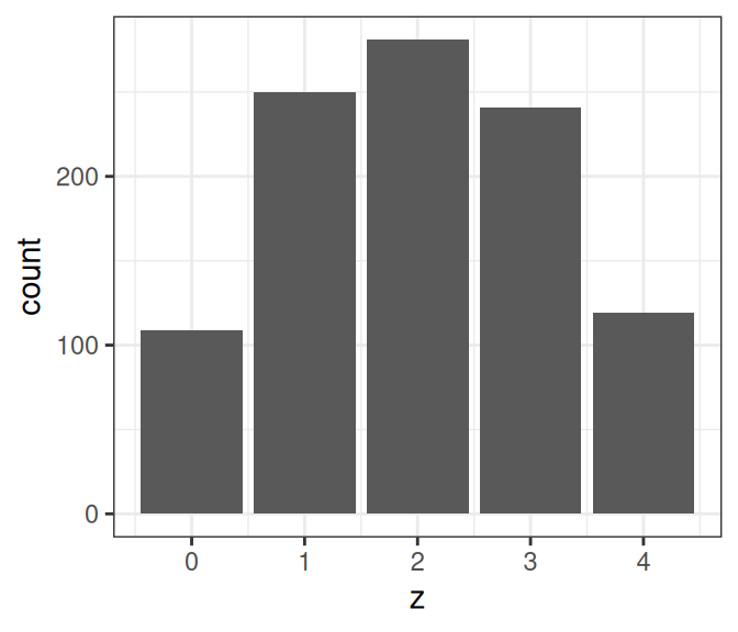
Prior Predictive Distribution

One way to check whether the prior is appropriate is to use the prior predictive distribution. Bayesian models are generative because they can be used to simulate data. The prior predictive distribution can be obtained by first simulating some $\theta$ values from the prior distribution and then simulating a data set for each $\theta$.

# Draw one theta
num_trials <- 4  # number of draws
sim_th1 <- sample(grid_df$th, size = 1,
                  # based on prior probability
                  prob = grid_df$pth)
# Simulate new data of four flips based on model
sim_y1 <- rbinom(num_trials, size = 1, prob = sim_th1)

# Repeat many times
# Set number of simulation draws
num_draws <- 1000
sim_th <- sample(grid_df$th, size = num_draws, replace = TRUE,
                 # based on prior probability
                 prob = grid_df$pth)
# Use a for loop
# Initialize output
sim_y <- matrix(NA, nrow = num_trials, ncol = num_draws)
for (s in seq_len(num_draws)) {
    # Store simulated data in the sth column
    sim_y[, s] <- rbinom(num_trials, size = 1, prob = sim_th[s])
}
# Show the first 10 simulated data sets based on prior:
sim_y[, 1:10]

#>      [,1] [,2] [,3] [,4] [,5] [,6] [,7] [,8] [,9] [,10]
#> [1,]    1    0    0    1    0    1    0    0    0     1
#> [2,]    0    0    0    1    1    0    1    0    1     1
#> [3,]    1    0    0    1    0    0    0    1    1     1
#> [4,]    1    0    1    1    1    0    0    1    1     0

# Show the distribution of number of heads
sim_heads <- colSums(sim_y)
ggplot(data.frame(z = sim_heads), aes(x = z)) +
    geom_bar()

The outcome seems to fit our intuition that it’s more likely to be half heads and half tails, but there is a lot of uncertainty.

3.5.3 Summarizing the Posterior

grid_df <- grid_df |>
    mutate(
        # Use our previously defined lik() function
        py_th = lik(th, num_flips = 4, num_heads = 1),
        # Product of prior and likelihood
        `prior x lik` = pth * py_th,
        # Scaled the posterior
        pth_y = `prior x lik` / sum(`prior x lik`)
    )
# Print a table
knitr::kable(grid_df)

th	pth	py_th	prior x lik	pth_y
0.00	0.00	0.0000000	0.0000000	0.0000000
0.05	0.01	0.0428687	0.0004287	0.0073359
0.10	0.02	0.0729000	0.0014580	0.0249500
0.15	0.03	0.0921188	0.0027636	0.0472914
0.20	0.04	0.1024000	0.0040960	0.0700927
0.25	0.05	0.1054688	0.0052734	0.0902416
0.30	0.06	0.1029000	0.0061740	0.1056525
0.35	0.07	0.0961187	0.0067283	0.1151381
0.40	0.08	0.0864000	0.0069120	0.1182815
0.45	0.09	0.0748688	0.0067382	0.1153071
0.50	0.10	0.0625000	0.0062500	0.1069530
0.55	0.09	0.0501187	0.0045107	0.0771891
0.60	0.08	0.0384000	0.0030720	0.0525695
0.65	0.07	0.0278687	0.0019508	0.0333832
0.70	0.06	0.0189000	0.0011340	0.0194056
0.75	0.05	0.0117188	0.0005859	0.0100268
0.80	0.04	0.0064000	0.0002560	0.0043808
0.85	0.03	0.0028687	0.0000861	0.0014727
0.90	0.02	0.0009000	0.0000180	0.0003080
0.95	0.01	0.0001187	0.0000012	0.0000203
1.00	0.00	0.0000000	0.0000000	0.0000000

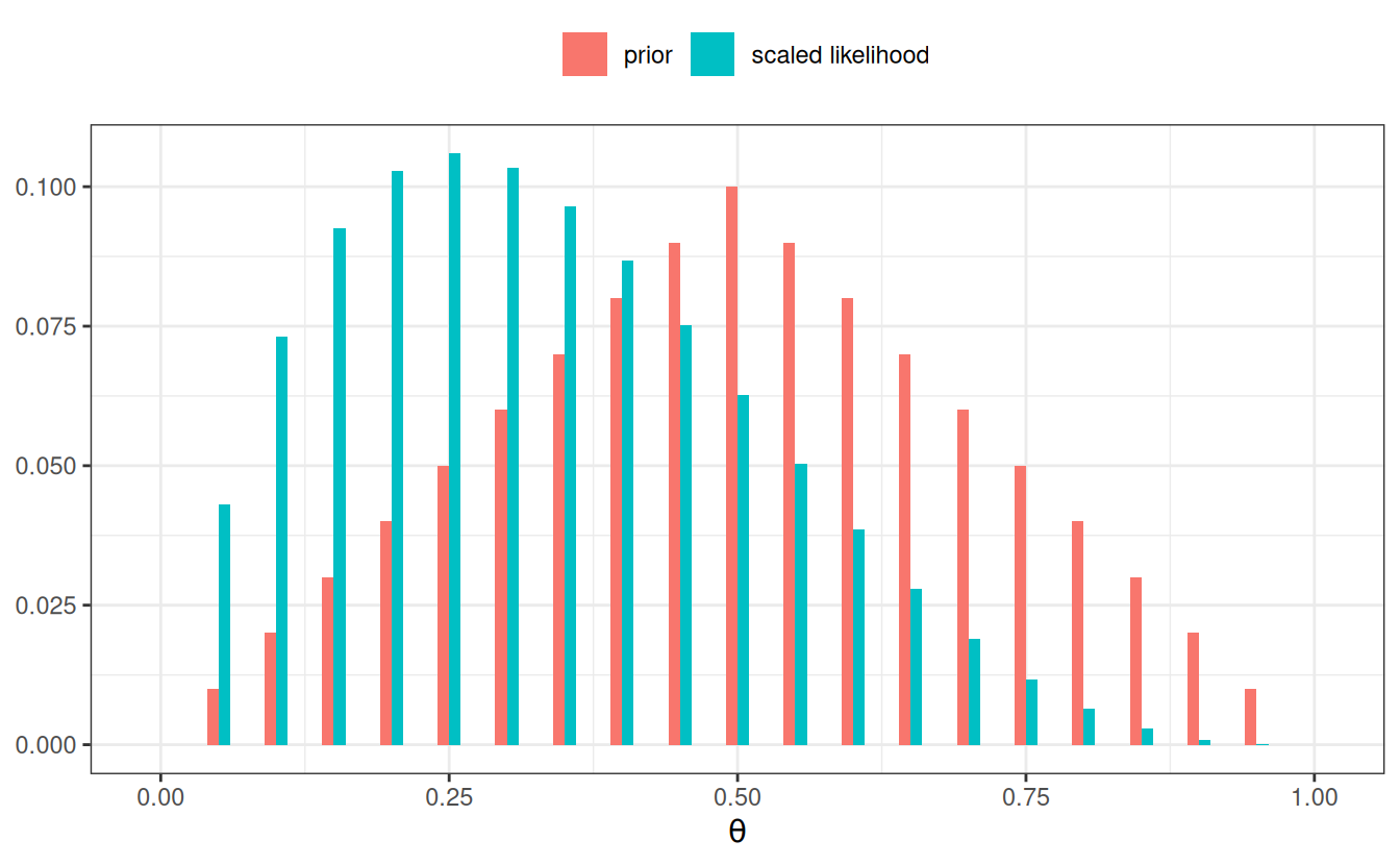
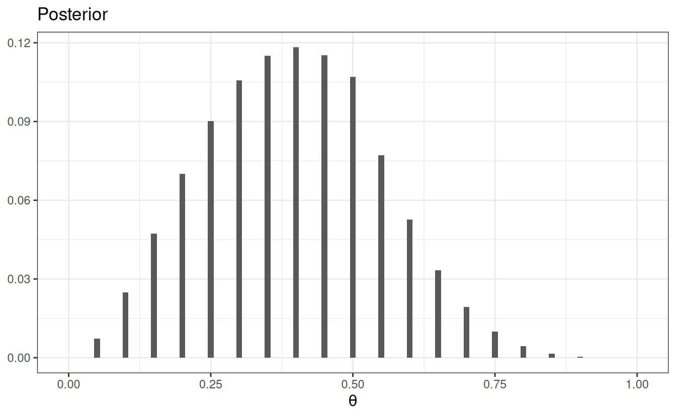
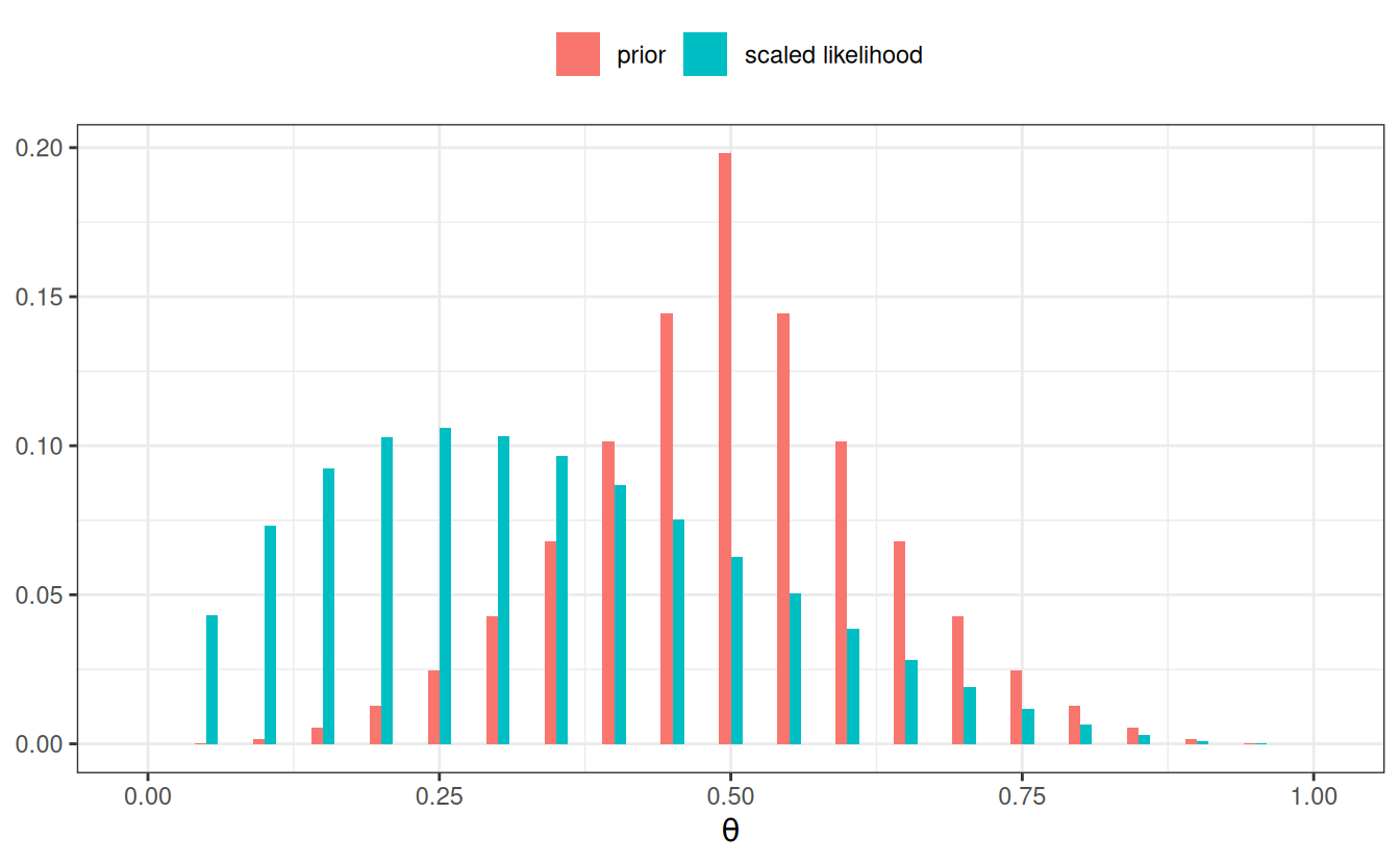
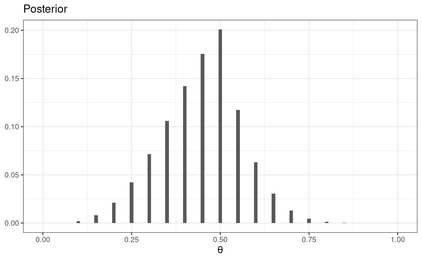
# Plot the prior/likelihood and the posterior
ggplot(data = grid_df, aes(x = th)) +
    geom_col(aes(x = th - 0.005, y = pth, fill = "prior"),
        width = 0.01,
    ) +
    geom_col(aes(x = th + 0.005, y = py_th / sum(py_th),
        fill = "scaled likelihood"), width = 0.01,
    ) +
    labs(fill = NULL, y = NULL, x = expression(theta)) +
    theme(legend.position = "top")
ggplot(data = grid_df, aes(x = th)) +
    geom_col(aes(x = th, y = pth_y), width = 0.01) +
    labs(
        fill = NULL, y = NULL, title = "Posterior",
        x = expression(theta)
    )

Figure 3.8 (b) shows the posterior distribution, which represents our updated belief about $\theta$. We can summarize it by simulating $\theta$ values from it and compute summary statistics:

# Define a function for computing posterior summary
summ_draw <- function(x) {
    c(
        mean = mean(x),
        median = median(x),
        sd = sd(x),
        mad = mad(x),
        `ci.1` = quantile(x, prob = .1, names = FALSE),
        `ci.9` = quantile(x, prob = .9, names = FALSE)
    )
}
# Sample from the posterior
post_samples <- sample(
    grid_df$th,
    size = 1000, replace = TRUE,
    prob = grid_df$pth_y
)
summ_draw(post_samples)

#>      mean    median        sd       mad      ci.1      ci.9 
#> 0.3848000 0.4000000 0.1538429 0.1482600 0.2000000 0.6000000

# Alternatively, use the `posterior` package
data.frame(theta = post_samples) |>
    posterior::summarize_draws()

Influence of Sample Size
Influence of Prior

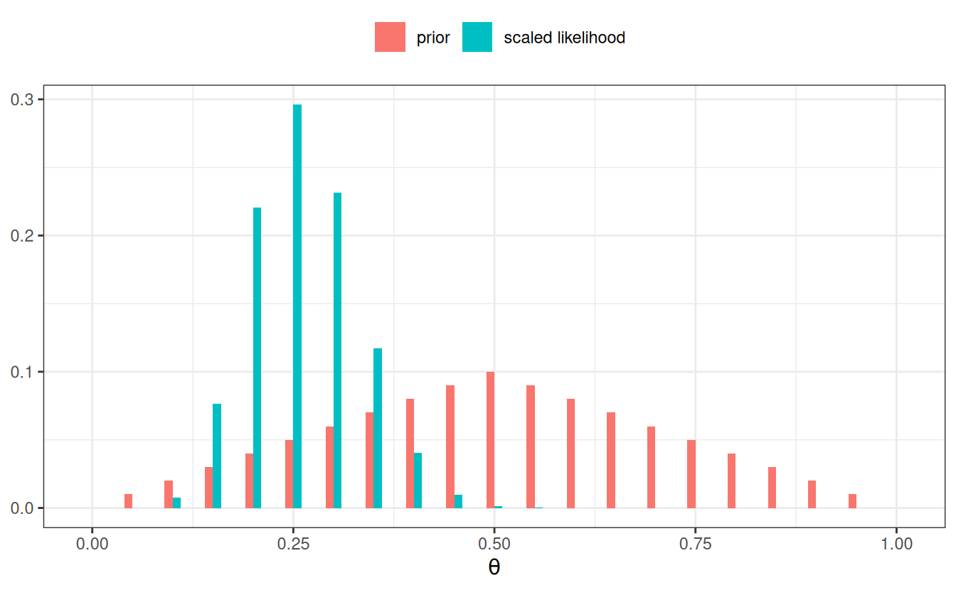
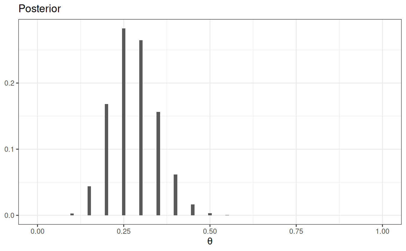
If, instead, we have $N$ = 40 and $z$ = 10, the posterior will be more similar to the likelihood.

grid_df2 <- grid_df |>
    mutate(
        # Use our previously defined lik() function
        py_th = lik(th, num_flips = 40, num_heads = 10),
        # Product of prior and likelihood
        `prior x lik` = pth * py_th,
        # Scaled the posterior
        pth_y = `prior x lik` / sum(`prior x lik`)
    )
# Plot the prior/likelihood and the posterior
ggplot(data = grid_df2, aes(x = th)) +
    geom_col(aes(x = th - 0.005, y = pth, fill = "prior"),
        width = 0.01,
    ) +
    geom_col(aes(x = th + 0.005, y = py_th / sum(py_th),
        fill = "scaled likelihood"), width = 0.01,
    ) +
    labs(fill = NULL, y = NULL, x = expression(theta)) +
    theme(legend.position = "top")

ggplot(data = grid_df2, aes(x = th)) +
    geom_col(aes(x = th, y = pth_y), width = 0.01) +
    labs(
        fill = NULL, y = NULL, title = "Posterior",
        x = expression(theta)
    )

# Sample from the posterior
post_samples <- sample(
    grid_df2$th,
    size = 1000, replace = TRUE,
    prob = grid_df2$pth_y
)
summ_draw(post_samples)

#>       mean     median         sd        mad       ci.1       ci.9 
#> 0.28085000 0.30000000 0.06542215 0.07413000 0.20000000 0.35000000

If we have a very strong prior concentrated at $\theta$ = .5, but still with $N$ = 40 and $z$ = 10, the posterior will be more similar to the prior.

grid_df3 <- grid_df |>
    mutate(
        # stronger prior
        pth = pth ^ 3,
        # scale the prior to sume to 1
        pth = pth / sum(pth),
        # Use our previously defined lik() function
        py_th = lik(th, num_flips = 4, num_heads = 1),
        # Product of prior and likelihood
        `prior x lik` = pth * py_th,
        # Scaled the posterior
        pth_y = `prior x lik` / sum(`prior x lik`)
    )
# Plot the prior/likelihood and the posterior
ggplot(data = grid_df3, aes(x = th)) +
    geom_col(aes(x = th - 0.005, y = pth, fill = "prior"),
        width = 0.01,
    ) +
    geom_col(aes(x = th + 0.005, y = py_th / sum(py_th),
        fill = "scaled likelihood"), width = 0.01,
    ) +
    labs(fill = NULL, y = NULL, x = expression(theta)) +
    theme(legend.position = "top")

ggplot(data = grid_df3, aes(x = th)) +
    geom_col(aes(x = th, y = pth_y), width = 0.01) +
    labs(
        fill = NULL, y = NULL, title = "Posterior",
        x = expression(theta)
    )

# Sample from the posterior
post_samples <- sample(
    grid_df3$th,
    size = 1000, replace = TRUE,
    prob = grid_df3$pth_y
)
summ_draw(post_samples)

#>      mean    median        sd       mad      ci.1      ci.9 
#> 0.4493000 0.4500000 0.1096656 0.0741300 0.3000000 0.6000000

# Alternatively, use the `posterior` package
data.frame(theta = post_samples) |>
    posterior::summarize_draws()

3.5.4 Remark on Grid Approximation

In this note, we discretized $\theta$ into a finite number of grid points to compute the posterior, mainly for pedagogical purposes. A big limitation is that our posterior will have no density for values other than the chosen grid points. While increasing the number of grid points (e.g., 1,000) can give more precision, the result is still not truly continuous. A bigger issue is that the computation breaks down when there is more than one parameter; if there are $p$ parameters, with 1,000 grid points per parameter, one needs to evaluate the posterior probability for $1,000^p$ grid points, which is not feasible even with modern computers. So more efficient algorithms, namely Markov chain Monte Carlo (MCMC) methods, will be introduced as we progress in the course.

The likelihood function in classical/frequentist statistics is usually written as $P(y; \theta)$. You will notice that here, I write the likelihood for classical/frequentist statistics to be different from the one used in Bayesian statistics. This is intentional: In frequentist conceptualization, $\theta$ is fixed, and it does not make sense to talk about the probability of $\theta$. This implies that we cannot condition on $\theta$, because conditional probability is defined only when $P(\theta)$ is defined.↩︎
The de Finetti’s theorem shows that when the data are exchangeable and can be considered an infinite sequence (i.e., not from a tiny finite population), then the data are conditionally independent given some $\theta$.↩︎

# Bayes's Theorem ```{r} #| label: setup #| include: false knitr::opts_chunk$set(comment = "#>") comma <- function(x, digits = 2L) format(x, digits = digits, big.mark = ",") # Load required packages library(tidyverse) theme_set(theme_bw() + theme(panel.grid.major.y = element_line(color = "grey92"))) ``` The Bayes's theorem is, surprisingly (or unsurprisingly), very simple: ::: {.callout-important appearance="simple" icon="false"} $$ P(B \mid A) = \frac{P(A \mid B) P(B)}{P(A)} $$ ::: More generally, we can expand it to incorporate the law of total probability to make it more applicable to data analysis. Consider $B_i$ as one of the $n$ many possible mutually exclusive events, then $$ \begin{aligned} P(B_i \mid A) & = \frac{P(A \mid B_i) P(B_i)}{P(A)} \\ & = \frac{P(A \mid B_i) P(B_i)} {P(A \mid B_1)P(B_1) + P(A \mid B_2)P(B_2) + \cdots + P(A \mid B_n)P(B_n)} \\ & = \frac{P(A \mid B_i) P(B_i)}{\sum_{k = 1}^n P(A \mid B_k)P(B_k)} \end{aligned} $$ If $B_i$ is a continuous variable, we will replace the sum by an integral, $$ P(B_i \mid A) = \frac{P(A \mid B_i) P(B_i)}{\int_k P(A \mid B_k)P(B_k)} $$ The denominator is not important for practical Bayesian analysis, therefore, it is sufficient to write the above equality as ::: {.callout-important appearance="simple" icon="false"} $$ P(B_i \mid A) \propto P(A \mid B_i) P(B_i) $$ ::: ## Example 1: Base rate fallacy (From Wikipedia) ::: {.panel-tabset} ### Question {.unnumbered} A police officer stops a driver *at random* and does a breathalyzer test for the driver. The breathalyzer is known to detect true drunkenness 100% of the time, but in 1% of the cases, it gives a false positive when the driver is sober. We also know that, in general, for every 1,000 drivers passing through that spot, one is driving drunk. Suppose that the breathalyzer shows positive for the driver. What is the probability that the driver is truly drunk? ### Solution {.unnumbered} $P(\text{positive} | \text{drunk}) = 1$ $P(\text{positive} | \text{sober}) = 0.01$ $P(\text{drunk}) = 1 / 1000$ $P(\text{sober}) = 999 / 1000$ Using Bayes' Theorem, $$ \begin{aligned} P(\text{drunk} | \text{positive}) & = \frac{P(\text{positive} | \text{drunk}) P(\text{drunk})} {P(\text{positive} | \text{drunk}) P(\text{drunk}) + P(\text{positive} | \text{sober}) P(\text{sober})} \\ & = \frac{1 \times 0.001}{1 \times 0.001 + 0.01 \times 0.999} \\ & = 100 / 1099 \approx 0.091 \end{aligned} $$ So there is less than a 10% chance that the driver is drunk even when the breathalyzer shows positive. You can verify that with a simulation using R: ```{r} #| label: sim-ex1 set.seed(4) truly_drunk <- c(rep("drunk", 100), rep("sober", 100 * 999)) table(truly_drunk) breathalyzer_test <- ifelse(truly_drunk == "drunk", # If drunk, 100% chance of showing positive "positive", # If not drunk, 1% chance of showing positive sample(c("positive", "negative"), 999000, replace = TRUE, prob = c(.01, .99) ) ) # Check the probability p(positive | sober) table(breathalyzer_test[truly_drunk == "sober"]) # 997 / 99900 = 0.00997998, so the error rate is less than 1% # Now, Check the probability p(drunk | positive) table(truly_drunk[breathalyzer_test == "positive"]) # 100 / (100 + 997) = 0.0911577, which is only 9.1%! ``` ::: ## Bayesian Statistics `Bayesian statistics` is a way to estimate some parameter $\theta$ (i.e., some quantities of interest, such as the population mean, regression coefficient, etc) by applying Bayes' Theorem. ::: {.callout-important appearance="simple" icon="false"} $$ P(\theta | D) \propto P(D | \theta) P(\theta) $$ ::: There are three components in the above equality: - $P(D | \theta)$, the probability that you observe data $D$, given the parameter $\theta$; this is called the `likelihood` (Note: It is the likelihood of $\theta$, but probability about $y$) - $P(\theta)$, the probability distribution $\theta$, without referring to the data $D$. This usually requires appeals to one's degree of belief, and so is called the *prior* - $P(\theta | y)$, the updated probability distribution of $\theta$, after observing the data $D$; this is called the *posterior* On the other hand, classical/frequentist statistics focuses solely on the likelihood function.[^lik] In Bayesian statistics, the goal is to update one's belief about $\theta$ based on the observed data $D$. [^lik]: The likelihood function in classical/frequentist statistics is usually written as $P(y; \theta)$. You will notice that here, I write the likelihood for classical/frequentist statistics to be different from the one used in Bayesian statistics. This is intentional: In frequentist conceptualization, $\theta$ is fixed, and it does not make sense to talk about the probability of $\theta$. This implies that we cannot condition on $\theta$, because conditional probability is defined only when $P(\theta)$ is defined. ## Example 2: Locating a Plane Consider a highly simplified scenario of locating a missing plane in the sea. Assume that we know the plane, before missing, happened to be flying at the same latitude, heading west across the Pacific, so we only need to find its longitude. We want to go out to collect debris (data) so that we can narrow the location ($\theta$) of the plane down. ::: {.panel-tabset} ### Prior We start with our prior. Assume that we have some rough idea where the plane should be, so we express our belief in a probability distribution like the following: ```{r} #| label: fig-prior-ex1 #| fig-cap: "Prior distribution." #| fig-width: 3 #| fig-asp: 0.8 #| echo: false dnorm_trunc <- function(x, mean = 0, sd = 1, ll = 0, ul = 1) { out <- dnorm(x, mean, sd) / (pnorm(ul, mean, sd) - pnorm(ll, mean, sd)) out[x > ul | x < ll] <- 0 out } ggplot(data.frame(x = c(0, 1)), aes(x = x)) + stat_function(fun = dnorm_trunc, args = list(mean = .8, sd = .5)) + ylim(0, 5) + labs(x = expression(location(theta)), y = "") + scale_x_continuous(breaks = c(0, 1), labels = c("West", "East")) ``` which says that our belief is that the plane is about twice more likely to be towards the east than towards the west. Below are two other options for priors (out of infinitely many), one providing virtually no information and the other encoding stronger information: ```{r} #| label: fig-more-prior-ex1 #| echo: false #| fig-asp: 0.8 #| fig-width: 3 #| fig-cap: "More options for prior distribution." #| fig-subcap: #| - "Noninformative prior." #| - "Informative prior." #| layout-ncol: 2 ggplot(data.frame(x = c(0, 1)), aes(x = x)) + stat_function(fun = dunif) + ylim(0, 5) + labs(x = expression(location(theta)), y = "") + scale_x_continuous(breaks = c(0, 1), labels = c("West", "East")) ggplot(data.frame(x = c(0, 1)), aes(x = x)) + stat_function(fun = dnorm_trunc, args = list(mean = .8, sd = .1)) + ylim(0, 5) + labs(x = expression(location(theta)), y = "") + scale_x_continuous(breaks = c(0, 1), labels = c("West", "East")) ``` The prior is chosen to reflect the researcher's belief, so different researchers will likely formulate a different prior for the same problem, and that's okay as long as the prior is reasonable and justified. Later, we will learn that in regular Bayesian analyses, with a moderate sample size, different priors generally only make negligible differences. ### Likelihood Now, assume that we have collected debris in the locations shown in the graph, ```{r} #| label: fig-likelihood-ex1 #| echo: false #| fig-width: 3 #| fig-asp: 0.8 qnorm_trunc <- function(p, mean = 0, sd = 1, ll = 0, ul = 1) { cdf_ll <- pnorm(ll, mean = mean, sd = sd) cdf_ul <- pnorm(ul, mean = mean, sd = sd) qnorm(cdf_ll + p * (cdf_ul - cdf_ll), mean = mean, sd = sd) } rnorm_trunc <- function(n, mean = 0, sd = 1, ll = 0, ul = 1) { p <- runif(n) qnorm_trunc(p, mean = mean, sd = sd, ll = ll, ul = ul) } grid <- seq(0, 1, length.out = 101) compute_lik <- function(x, pts = grid, sd = 0.2, binwidth = .01) { lik_vals <- vapply(x, dnorm_trunc, mean = pts, sd = sd, FUN.VALUE = numeric(length(pts)) ) lik <- apply(lik_vals, 1, prod) lik / sum(lik) / binwidth } set.seed(4) dat_x <- rnorm_trunc(10, mean = 0.6, sd = 0.2) lik_x <- compute_lik(dat_x) ggplot( data.frame(x = grid, dens = lik_x), aes(x = x, y = dens) ) + geom_line() + geom_point( data = data.frame(x = dat_x), aes(x = x), y = 0, shape = 1, col = "red" ) + labs(y = "Likelihood (Scaled)", x = expression(location(theta))) + scale_x_continuous(breaks = c(0, 1), labels = c("West", "East")) ``` ### Posterior Now, from Bayes's Theorem, $$ \text{Posterior Probability} \propto \text{Prior Probability} \times \text{Likelihood} $$ So we can simply multiply the prior probabilities and the likelihood to get the posterior probability for every location. A rescaling step is needed to ensure that the area under the curve will be 1, which is usually performed by the software. ```{r} #| label: fig-posterior-ex1 #| echo: false #| fig-width: 4 #| fig-asp: 0.618 update_probs <- function(prior_probs, lik, binwidth = .01) { post_probs <- prior_probs * lik post_probs / sum(post_probs) / binwidth } ggplot(data.frame(x = c(0, 1)), aes(x = x)) + stat_function( fun = dnorm_trunc, args = list(mean = .8, sd = .5), aes(linetype = "Prior", col = "Prior") ) + geom_line( data = data.frame(x = grid, dens = lik_x), aes( x = x, y = dens, linetype = "Likelihood", col = "Likelihood" ) ) + geom_line( data = data.frame( x = grid, dens = update_probs( dnorm_trunc(grid, .8, .5), lik_x ) ), aes(x = x, y = dens, col = "Posterior", linetype = "Posterior") ) + ylim(0, 7) + labs(x = expression(location(theta)), y = "") + scale_x_continuous(breaks = c(0, 1), labels = c("West", "East")) + scale_color_manual("", values = c("red", "blue", "black")) + scale_linetype_manual("", values = c("twodash", "solid", "dashed")) ``` ::: As illustrated below, the posterior distribution is a synthesis of (a) the prior and (b) the data (likelihood). ::: {.panel-tabset} ### Influence of Prior @fig-posterior-ex1-prior shows what happen with a stronger prior: ```{r} #| label: fig-posterior-ex1-prior #| echo: false #| fig-width: 4 #| fig-asp: 0.618 ggplot(data.frame(x = c(0, 1)), aes(x = x)) + stat_function( fun = dnorm_trunc, args = list(mean = .8, sd = .1), aes(linetype = "Prior", col = "Prior") ) + geom_line( data = data.frame(x = grid, dens = lik_x), aes( x = x, y = dens, linetype = "Likelihood", col = "Likelihood" ) ) + geom_line( data = data.frame( x = grid, dens = update_probs( dnorm_trunc(grid, .8, .1), lik_x ) ), aes(x = x, y = dens, col = "Posterior", linetype = "Posterior") ) + ylim(0, 7) + labs(x = expression(location(theta)), y = "") + scale_x_continuous(breaks = c(0, 1), labels = c("West", "East")) + scale_color_manual("", values = c("red", "blue", "black")) + scale_linetype_manual("", values = c("twodash", "solid", "dashed")) ``` ### Influence of More Data @fig-posterior-ex1-data shows what happen with 20 more data points: ```{r} #| label: fig-posterior-ex1-data #| echo: false #| fig-width: 4 #| fig-asp: 0.618 dat_x <- c(dat_x, rnorm_trunc(20, mean = 0.6, sd = 0.2)) lik_x <- compute_lik(dat_x) ggplot(data.frame(x = c(0, 1)), aes(x = x)) + stat_function( fun = dnorm_trunc, args = list(mean = .8, sd = .1), aes(linetype = "Prior", col = "Prior") ) + geom_line( data = data.frame(x = grid, dens = lik_x), aes( x = x, y = dens, linetype = "Likelihood", col = "Likelihood" ) ) + geom_line( data = data.frame( x = grid, dens = update_probs( dnorm_trunc(grid, .8, .1), lik_x ) ), aes(x = x, y = dens, col = "Posterior", linetype = "Posterior") ) + ylim(0, 20) + labs(x = expression(location(theta)), y = "") + scale_x_continuous(breaks = c(0, 1), labels = c("West", "East")) + scale_color_manual("", values = c("red", "blue", "black")) + scale_linetype_manual("", values = c("twodash", "solid", "dashed")) ``` ::: ## Data-Order Invariance In many data analysis applications, researchers collect some data $D_1$, and then collect some more data $D_2$. An example would be researchers conducting two separate experiments to study the same research question. In Bayesian statistics, one can consider three ways to obtain the posterior: 1. Update the belief with $D_1$, and then with $D_2$ 2. Update the belief with $D_2$, and then with $D_1$ 3. Update the belief with both $D_1$ and $D_2$ simultaneously Whether these three ways give the same posterior depends on whether **data-order invariance** holds. If the inference of $D_1$ does not depend on $D_2$, or vice versa, then all three ways lead to the same posterior. Specifically, if we have **conditional independence** such that $$ P(D_1, D_2 \mid \theta) = P(D_1 \mid \theta) P(D_2 \mid \theta), $$ then one can show all three ways give the same posterior [[see section 4.4 and 4.5 of @johnson2022]](https://www.bayesrulesbook.com/chapter-4#ch4-sequential). ::: {.callout-tip} ## Exchangeability* Exchangeability is an important concept in Bayesian statistics. Data are exchangeable when the joint distribution, $P(D_1, \ldots, D_N)$, does not depend on the ordering of the data. A simple way to think about it is if you scramble the order of your outcome variable in your data set and still can obtain the same statistical results, then the data are exchangeable. An example situation where data are not exchangeable is - $D_1$ is from year 1990, $D_2$ is from year 2020, and the parameter $\theta$ changes from 1990 to 2020 When data are exchangeable, conditional independence would generally hold.[^deFinetti] [^deFinetti]: The [de Finetti's theorem](https://en.wikipedia.org/wiki/De_Finetti%27s_theorem) shows that when the data are exchangeable and can be considered an infinite sequence (i.e., not from a tiny finite population), then the data are conditionally independent given some $\theta$. ::: ## Bernoulli Likelihood For binary data $y$ (e.g., coin flip, pass/fail, diagnosed/not), an intuitive way to analyze is to use a Bernoulli model: $$ \begin{aligned} P(y = 1 \mid \theta) = \theta \\ P(y = 0 \mid \theta) = 1 - \theta \end{aligned}, $$ which is more compactly written as $$ P(y \mid \theta) = \theta^y (1 - \theta)^{(1 - y)}, $$ where $\theta \in [0, 1]$ is the probability of a "1". You can verify that the compact form is the same as the longer form. ### Multiple Observations When there are more than one $y$, say $y_1, \ldots, y_N$, that are conditionally independent, we have $$ \begin{aligned} P(y_1, \ldots, y_N \mid \theta) & = \prod_{i = 1}^N P(y_i \mid \theta) \\ & = \theta^{\sum_{i = 1}^N y_i} (1 - \theta)^{\sum_{i = 1}^N (1 - y_i)} \\ & = \theta^z (1 - \theta)^{N - z} \end{aligned}, $$ where $z$ is the number of "1"s (e.g., the number of heads in coin flips). Note that the likelihood only depends on $z$, not the individual $y$s. In other words, the likelihood is the same as long as there are $z$ heads, regardless of when those heads occur. Let's say $N$ = 4 and $z$ = 1. We can plot the likelihood in R: ```{r} #| label: fig-lik #| fig-width: 3.5 #| fig-height: 3 #| fig-cap: Binomial likelihood function with $N$ = 4 and $z$ = 1 # Write the likelihood as a function of theta lik <- function(th, num_flips = 4, num_heads = 1) { th ^ num_heads * (1 - th) ^ (num_flips - num_heads) } # Likelihood of theta = 0.5 lik(0.5) # Plot the likelihood ggplot(data.frame(th = c(0, 1)), aes(x = th)) + # `stat_function` for plotting a function stat_function(fun = lik) + # use `expression()` to get greek letters labs(x = expression(theta), y = "Likelihood with N = 4 and z = 1") ``` ### Setting Priors Remember again the relationship between the prior and the posterior: $$P(\theta | y) \propto P(y | \theta) P(\theta)$$ The posterior distributions are mathematically determined once the priors and the likelihood are set. However, the mathematical form of the posterior is sometimes very difficult to deal with. One straightforward, brute-force method is to discretize the parameter space into a number of points. For example, by taking $\theta$ = 0, 0.05, 0.10, . . . , 0.90, 0.95, 1.00, one can evaluate the posterior at these 21 **grid points**. Let's use a prior that peaks at 0.5 and linearly decreases to both sides. I assume that $\theta$ = 0.5 is twice as likely as $\theta = 0.25$ or $\theta = 0.75$ to reflect my belief that the coin is more likely to be fair. ```{r} #| label: grid_df-prior # Define a grid for the parameter grid_df <- data.frame(th = seq(0, 1, by = 0.05)) # Set the prior mass for each value on the grid grid_df$pth <- c(0:10, 9:0) # linearly increasing, then decreasing # Convert pth to a proper distribution such that the value # sum to one grid_df$pth <- grid_df$pth / sum(grid_df$pth) # <1> # Plot the prior ggplot(grid_df, aes(x = th, y = pth)) + geom_col(aes(x = th, y = pth), width = 0.01, ) + labs(y = expression(P(theta)), x = expression(theta)) ``` 1. This line ensures that the probability values sum to one. This is a trick we will use to obtain the posterior probability. ::: {.callout-important appearance="minimal"} ### Prior Predictive Distribution One way to check whether the prior is appropriate is to use the **prior predictive distribution**. Bayesian models are **generative** because they can be used to simulate data. The prior predictive distribution can be obtained by first simulating some $\theta$ values from the prior distribution and then simulating a data set for each $\theta$. ```{r} #| label: prior-predictive #| fig-width: 3.5 #| fig-height: 3 # Draw one theta num_trials <- 4 # number of draws sim_th1 <- sample(grid_df$th, size = 1, # based on prior probability prob = grid_df$pth) # Simulate new data of four flips based on model sim_y1 <- rbinom(num_trials, size = 1, prob = sim_th1) # Repeat many times # Set number of simulation draws num_draws <- 1000 sim_th <- sample(grid_df$th, size = num_draws, replace = TRUE, # based on prior probability prob = grid_df$pth) # Use a for loop # Initialize output sim_y <- matrix(NA, nrow = num_trials, ncol = num_draws) for (s in seq_len(num_draws)) { # Store simulated data in the sth column sim_y[, s] <- rbinom(num_trials, size = 1, prob = sim_th[s]) } # Show the first 10 simulated data sets based on prior: sim_y[, 1:10] # Show the distribution of number of heads sim_heads <- colSums(sim_y) ggplot(data.frame(z = sim_heads), aes(x = z)) + geom_bar() ``` The outcome seems to fit our intuition that it's more likely to be half heads and half tails, but there is a lot of uncertainty. ::: ### Summarizing the Posterior ```{r} #| label: grid_df-post grid_df <- grid_df |> mutate( # Use our previously defined lik() function py_th = lik(th, num_flips = 4, num_heads = 1), # Product of prior and likelihood `prior x lik` = pth * py_th, # Scaled the posterior pth_y = `prior x lik` / sum(`prior x lik`) ) # Print a table knitr::kable(grid_df) ``` ```{r} #| label: fig-grid-post #| fig-asp: 0.618 #| fig-cap: Bernoulli posterior distribution #| fig-subcap: #| - Prior and likelihood #| - Posterior #| layout-nrow: 2 # Plot the prior/likelihood and the posterior ggplot(data = grid_df, aes(x = th)) + geom_col(aes(x = th - 0.005, y = pth, fill = "prior"), width = 0.01, ) + geom_col(aes(x = th + 0.005, y = py_th / sum(py_th), fill = "scaled likelihood"), width = 0.01, ) + labs(fill = NULL, y = NULL, x = expression(theta)) + theme(legend.position = "top") ggplot(data = grid_df, aes(x = th)) + geom_col(aes(x = th, y = pth_y), width = 0.01) + labs( fill = NULL, y = NULL, title = "Posterior", x = expression(theta) ) ``` @fig-grid-post-2 shows the posterior distribution, which represents our updated belief about $\theta$. We can summarize it by simulating $\theta$ values from it and compute summary statistics: ```{r} #| label: summarize-post-draws # Define a function for computing posterior summary summ_draw <- function(x) { c( mean = mean(x), median = median(x), sd = sd(x), mad = mad(x), `ci.1` = quantile(x, prob = .1, names = FALSE), `ci.9` = quantile(x, prob = .9, names = FALSE) ) } # Sample from the posterior post_samples <- sample( grid_df$th, size = 1000, replace = TRUE, prob = grid_df$pth_y ) summ_draw(post_samples) # Alternatively, use the `posterior` package data.frame(theta = post_samples) |> posterior::summarize_draws() ``` ::: {.panel-tabset} ### Influence of Sample Size If, instead, we have $N$ = 40 and $z$ = 10, the posterior will be more similar to the likelihood. ```{r} #| label: grid_df-2 #| fig.asp: 0.618 grid_df2 <- grid_df |> mutate( # Use our previously defined lik() function py_th = lik(th, num_flips = 40, num_heads = 10), # Product of prior and likelihood `prior x lik` = pth * py_th, # Scaled the posterior pth_y = `prior x lik` / sum(`prior x lik`) ) # Plot the prior/likelihood and the posterior ggplot(data = grid_df2, aes(x = th)) + geom_col(aes(x = th - 0.005, y = pth, fill = "prior"), width = 0.01, ) + geom_col(aes(x = th + 0.005, y = py_th / sum(py_th), fill = "scaled likelihood"), width = 0.01, ) + labs(fill = NULL, y = NULL, x = expression(theta)) + theme(legend.position = "top") ggplot(data = grid_df2, aes(x = th)) + geom_col(aes(x = th, y = pth_y), width = 0.01) + labs( fill = NULL, y = NULL, title = "Posterior", x = expression(theta) ) ``` ```{r} #| label: summarize-post-draws-2 # Sample from the posterior post_samples <- sample( grid_df2$th, size = 1000, replace = TRUE, prob = grid_df2$pth_y ) summ_draw(post_samples) ``` ### Influence of Prior If we have a very strong prior concentrated at $\theta$ = .5, but still with $N$ = 40 and $z$ = 10, the posterior will be more similar to the prior. ```{r} #| label: grid_df-3 #| fig-asp: 0.618 grid_df3 <- grid_df |> mutate( # stronger prior pth = pth ^ 3, # scale the prior to sume to 1 pth = pth / sum(pth), # Use our previously defined lik() function py_th = lik(th, num_flips = 4, num_heads = 1), # Product of prior and likelihood `prior x lik` = pth * py_th, # Scaled the posterior pth_y = `prior x lik` / sum(`prior x lik`) ) # Plot the prior/likelihood and the posterior ggplot(data = grid_df3, aes(x = th)) + geom_col(aes(x = th - 0.005, y = pth, fill = "prior"), width = 0.01, ) + geom_col(aes(x = th + 0.005, y = py_th / sum(py_th), fill = "scaled likelihood"), width = 0.01, ) + labs(fill = NULL, y = NULL, x = expression(theta)) + theme(legend.position = "top") ggplot(data = grid_df3, aes(x = th)) + geom_col(aes(x = th, y = pth_y), width = 0.01) + labs( fill = NULL, y = NULL, title = "Posterior", x = expression(theta) ) ``` ```{r} #| label: summarize-post-draws-3 # Sample from the posterior post_samples <- sample( grid_df3$th, size = 1000, replace = TRUE, prob = grid_df3$pth_y ) summ_draw(post_samples) # Alternatively, use the `posterior` package data.frame(theta = post_samples) |> posterior::summarize_draws() ``` ::: ### Remark on Grid Approximation In this note, we discretized $\theta$ into a finite number of grid points to compute the posterior, mainly for pedagogical purposes. A big limitation is that our posterior will have no density for values other than the chosen grid points. While increasing the number of grid points (e.g., 1,000) can give more precision, the result is still not truly continuous. A bigger issue is that the computation breaks down when there is more than one parameter; if there are $p$ parameters, with 1,000 grid points per parameter, one needs to evaluate the posterior probability for $1,000^p$ grid points, which is not feasible even with modern computers. So more efficient algorithms, namely Markov chain Monte Carlo (MCMC) methods, will be introduced as we progress in the course.