Generalizability Theory
Learning Objectives
- Provide some example applications of the generalizability theory (G theory)
- Contrast G theory with CTT (Table 10.1)
- Explain the differences between crossed and nested facets, and between random and fixed facets, and between G studies and D studies
- Estimate variance components and the G and \(\phi\) coefficients for two facets designs
library(here)
library(haven)  # for reading SPSS data
library(tidyverse)
library(lme4)
Basic Concepts of G theory
Premise: there are multiple sources of error, and typically observed scores only reflect some specific conditions (e.g., one rater, two trials)
Goal: investigate whether observed scores under one set of conditions can be generalized to broader conditions.
Common Applications
- Rating data. Interrater reliability is a special case of G theory.
- Behavioral observations: generalizability across different raters, tasks, occasions, intervals of observations, etc.
- Imaging data: generalizability of scores across different processing decisions, tasks, etc.
Terminology
Facet: sources of error (e.g., raters, tasks, occasions). Each facet can be fixed or random.
Condition: level of a facet
Object of Measurement: usually people, which is not considered a facet. This is always random.
Universe of Admissible Operations (UAO): a broad set of conditions to which the observed scores generalize
Universerse Score: average score of a person across all possible sets of conditions in the UAO
G Study: obtain accurate information on the magnitude of sources of error
D study: design measurement scenario with the desired level of dependability with the smallest number of conditions
In G theory, by evaluating the degree of error in different sources, we have evidence on whether scores from some admissible conditions are generalizable across conditions. If so, the scores are dependable (or reliable).
One-Facet Design
The example in the previous note with each participant rated by the same set of raters is an example of a one-facet design.
Formula for score of person \(i\) by rater \(j\):
\[ \begin{aligned} Y_{ij} & = \mu & \text{(universe score)} \\ & \quad + (\mu_p - \mu) & \text{(person effect)} \\ & \quad + (\mu_r - \mu) & \text{(rater effect)} \\ & \quad + (Y_{ij} - \mu_p - \mu_r + \mu) & \text{(residual)} \end{aligned} \]
This gives the variance decomposition for three components:
\[\sigma^2(Y_{pr}) = \sigma^2_p + \sigma^2_r + \sigma^2_{pr, e}\]
\(\sigma^2_p\) is person variance, or universe score variance.
Model of analysis: two-way random-effect ANOVA, aka random-effect model, variance component models, or multilevel models with crossed random effects.
Two-Facet Design
The first example comes from the companion website of the textbook, which can be downloaded here: https://www.guilford.com/companion-site/Measurement-Theory-and-Applications-for-the-Social-Sciences/9781462532131
The file you need is the SPSS zip file from Chapter 10.
# Import data
# Assume you downloaded the data to the folder "data", with the name
# "Bandalos_Ch10_SPSS.zip"
zip_data <- here("data", "Bandalos_Ch10_SPSS.zip")
sample_data <- read_sav(
    unz(zip_data,
        "Bandalos_Ch10_SPSS/Data/Table 10.4 data untransposed.sav")
)
sample_data
Data Transformation
The data are in a typical wide format.
- Each row represents a person
- The other facets (rater, task) are embedded in the columns
While it’s possible to run analyses using the wide format, for our analyses we’ll transform the data to a long format as it better suits the analytic framework (variance components model) we’ll use. This also has better handling for missing data.
We’ll use the pivot_longer() function from the tidyr package (which is loaded with library(tidyverse)).
sample_long <- pivot_longer(
    sample_data,
    # select all columns, except the 1st one to be transformed
    cols = -1,
    # The columns have a pattern "R(1)Task(2)", where values
    # in parentheses are the IDs for the facets. So we first
    # specify this pattern, with a "." meaning a one-digit
    # place holder,
    names_pattern = "R(.)Task(.)",
    # and then specify that the first place holder is for rater,
    # and the second place-holder is for task.
    names_to = c("rater", "task"),
    values_to = "score"  # name of score variable
)
head(sample_long)
As can be seen, the data are now in a long format.
- Each row represents an observation (repeated measure)
- Each facet (rater, task) has its own column
Nested vs. Crossed
Crossed Design
The data here has each participant (p) rated by the same three raters (r) on each of the three tasks (t). Therefore, this is a p \(\times\) r \(\times\) t design, where the two facets are crossed. We can see this by looking at the following tables:
with(sample_long,
     table(person, rater))
rater
person 1 2 3
1 3 3 3
2 3 3 3
3 3 3 3
4 3 3 3
5 3 3 3
6 3 3 3
7 3 3 3
8 3 3 3
9 3 3 3
10 3 3 3
11 3 3 3
12 3 3 3with(sample_long,
table(rater, task)) task
rater 1 2 3
1 12 12 12
2 12 12 12
3 12 12 12with(sample_long,
table(person, task)) task
person 1 2 3
1 3 3 3
2 3 3 3
3 3 3 3
4 3 3 3
5 3 3 3
6 3 3 3
7 3 3 3
8 3 3 3
9 3 3 3
10 3 3 3
11 3 3 3
12 3 3 3With a crossed (factorial) design, every cell should be filled.
Nested Design
On the other hand, if we have different sets of raters for different tasks, we will have a nested design. Let’s say we actually have 9 raters, with raters 1-3 for task 1, raters 4-6 for task 2, and raters 7-9 for task 3. This yields a p \(\times\) (r:t) design with raters nested within tasks.
# Recode raters
sample2 <- sample_long |>
    group_by(person) |>
    mutate(actual_rater = 1:9) |>
    ungroup()
with(sample2,
     table(person, actual_rater))
actual_rater
person 1 2 3 4 5 6 7 8 9
1 1 1 1 1 1 1 1 1 1
2 1 1 1 1 1 1 1 1 1
3 1 1 1 1 1 1 1 1 1
4 1 1 1 1 1 1 1 1 1
5 1 1 1 1 1 1 1 1 1
6 1 1 1 1 1 1 1 1 1
7 1 1 1 1 1 1 1 1 1
8 1 1 1 1 1 1 1 1 1
9 1 1 1 1 1 1 1 1 1
10 1 1 1 1 1 1 1 1 1
11 1 1 1 1 1 1 1 1 1
12 1 1 1 1 1 1 1 1 1with(sample2,
table(actual_rater, task)) task
actual_rater 1 2 3
1 12 0 0
2 0 12 0
3 0 0 12
4 12 0 0
5 0 12 0
6 0 0 12
7 12 0 0
8 0 12 0
9 0 0 12with(sample2,
table(person, task)) task
person 1 2 3
1 3 3 3
2 3 3 3
3 3 3 3
4 3 3 3
5 3 3 3
6 3 3 3
7 3 3 3
8 3 3 3
9 3 3 3
10 3 3 3
11 3 3 3
12 3 3 3When facet A is nested in facet B (i.e., a:b), each level of A is associated with only one level of B, but each level of B is associated with multiple levels of A.
Variance Decomposition
With a two-facet crossed design, we have the following variance components:
- Person
- Facet A
- Facet B
- Person \(\times\) A
- Person \(\times\) B
- A \(\times\) B
- Person \(\times\) A \(\times\) B*
- Error*
*The variances due to Person \(\times\) A \(\times\) B interaction and random error can only be separated when there is more than one observation for each cell (i.e., combination of person, A, and B), which is uncommon.
m1 <- lmer(
    score ~ 1 +
        (1 | person) + (1 | rater) + (1 | task) +
        (1 | person:rater) + (1 | person:task) +
        (1 | rater:task),
    data = sample_long
)
boundary (singular) fit: see help('isSingular')# Variance components (VCs)
vc_m1 <- as.data.frame(VarCorr(m1))
# Organize in a table, similar to Table 10.4
data.frame(source = vc_m1$grp,
var = vc_m1$vcov,
percent = vc_m1$vcov / sum(vc_m1$vcov))Bootstrap Standard Errors and Confidence Intervals
get_vc <- function(x) {
    vc_x <- as.data.frame(VarCorr(x))
    c(vc_x$vcov, vc_x$vcov / sum(vc_x$vcov))
}
boo <- bootMer(m1, FUN = get_vc, nsim = 1999)
# Get percentile CIs for person variance
boot::boot.ci(boo, type = "perc", index = 3)
BOOTSTRAP CONFIDENCE INTERVAL CALCULATIONS
Based on 1999 bootstrap replicates
CALL :
boot::boot.ci(boot.out = boo, type = "perc", index = 3)
Intervals :
Level Percentile
95% ( 0.162, 2.366 )
Calculations and Intervals on Original Scale# Get percentile CIs for proportion of person variance
boot::boot.ci(boo, type = "perc", index = 10)BOOTSTRAP CONFIDENCE INTERVAL CALCULATIONS
Based on 1999 bootstrap replicates
CALL :
boot::boot.ci(boot.out = boo, type = "perc", index = 10)
Intervals :
Level Percentile
95% ( 0.1112, 0.6730 )
Calculations and Intervals on Original Scale# Get percentile CIs for all VCs
ci_vc <- lapply(1:14, FUN = function(i) {
ci_i <- boot::boot.ci(boo, type = "perc", index = i)$percent
c(ll_var = ci_i[4], ul_var = ci_i[5])
})It also helps to create a function so that we can do the same operation in the future:
table_vc <- function(x, digits = 2) {
    vc_x <- as.data.frame(VarCorr(x))
    out <- data.frame(
        source = vc_x$grp,
        sd = sqrt(vc_x$vcov),
        var = vc_x$vcov,
        percent = vc_x$vcov / sum(vc_x$vcov))
    print(out, digits = digits)
}
table_vc(m1)
source sd var percent
1 person:task 0.35 0.119 0.0511
2 person:rater 0.68 0.468 0.2003
3 person 1.02 1.036 0.4432
4 rater:task 0.11 0.012 0.0049
5 task 0.25 0.061 0.0262
6 rater 0.00 0.000 0.0000
7 Residual 0.80 0.641 0.2743# Add CIs
cbind(table_vc(m1),
do.call(rbind, ci_vc[1:7]),
prop = do.call(rbind, ci_vc[8:14])) |>
print(digits = 2) source sd var percent
1 person:task 0.35 0.119 0.0511
2 person:rater 0.68 0.468 0.2003
3 person 1.02 1.036 0.4432
4 rater:task 0.11 0.012 0.0049
5 task 0.25 0.061 0.0262
6 rater 0.00 0.000 0.0000
7 Residual 0.80 0.641 0.2743
source sd var percent ll_var ul_var prop.ll_var prop.ul_var
1 person:task 0.35 0.119 0.0511 0.00 0.364 0.000 0.173
2 person:rater 0.68 0.468 0.2003 0.11 0.919 0.049 0.413
3 person 1.02 1.036 0.4432 0.16 2.366 0.111 0.673
4 rater:task 0.11 0.012 0.0049 0.00 0.097 0.000 0.047
5 task 0.25 0.061 0.0262 0.00 0.306 0.000 0.134
6 rater 0.00 0.000 0.0000 0.00 0.156 0.000 0.076
7 Residual 0.80 0.641 0.2743 0.40 0.889 0.142 0.472As shown above, while universe score variance (person variance) is the largest, it only accounts for a proportion of 0.4431584 of the total variance. If we use teminology analogous to classical test theory, it means that if we use a single rating of a single task to generalize to the universe score, less than half of the observed score variance is due to true score variance.
Interpreting the Variance Components
Venn diagrams
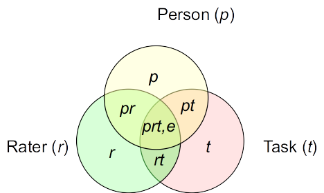

Standard deviation
E.g., The ratings are on a 6-point scale. With \(\hat \sigma_{pr}\) = 0.6841528, this is the margin of error due to rater-by-person interaction, which is not trivial.
Fixed vs. Random
Generally G theory treats conditions of a facet as random, meaning they are regarded as a random sample from a population collection of samples. However, if such an assumption does not make sense, such as when people are always going to be evaluated on the same tasks, and there is no intention to generalize beyond those tasks, the task facet should be treated as fixed. Then there are two options:
If it makes sense to average the different conditions in a fixed facet (e.g., average score across tasks), follow the code below.
Otherwise, perform a separate G study for each condition of the fixed facet.
# If treating task as fixed, the person x task variance will be averaged
# and become part of the universe score
varu <- vc_m1$vcov[3] + vc_m1$vcov[1] / 3
# The rater x task variance will be averaged and become part of rater variance
varr <- vc_m1$vcov[6] + vc_m1$vcov[4] / 3
# The residual will be averaged and become part of person x rater variance
vare <- vc_m1$vcov[2] + vc_m1$vcov[7] / 3
# Combine
data.frame(source = vc_m1$grp[c(3, 6, 2)],
           var = c(varu, varr, vare),
           percent = c(varu, varr, vare) / sum(varu, varr, vare))
Relative vs. Absolute Decisions
Error for relative: anything that involves person, including the residual
Error for absolute: every term other than person
D Studies
Decision studies: Based on the results of G studies, try to minimize error as much as possible.
- Find out how many conditions can be used to optimize generalizability
- Similar to using the Spearman-Brown prophecy formula, but consider multiple sources of errors
G and \(\phi\) Coefficients
G coefficient: For relative decisions
- Only include sources of variation that would change relative standing as error (\(\sigma^2_\text{REL}\))
- i.e., interaction terms that involve persons
\[G = \frac{\hat \sigma^2_p}{\hat \sigma^2_p + \hat \sigma^2_\text{REL}}\]
\(\phi\) coefficient: For absolute decisions
- Include all sources of variation, except for the one due to persons, as error (\(\sigma^2_\text{ABS}\))
\[\phi = \frac{\hat \sigma^2_p}{\hat \sigma^2_p + \hat \sigma^2_\text{ABS}}\]
These are analogous to reliability coefficients.
mean_scores <- rowMeans(sample_data[-1])
dep_coef <- function(x) {
    vc_x <- as.data.frame(VarCorr(x))
    # G coefficient (for relative decision)
    g_coef <- with(
        vc_x,
        vcov[3] / (vcov[3] + vcov[1] / 3 + vcov[2] / 3 + vcov[7] / 3 / 3)
    )
    # phi coefficient (for absolute decision)
    phi_coef <- with(
        vc_x,
        vcov[3] /
            (vcov[3] + vcov[1] / 3 + vcov[2] / 3 +
             vcov[7] / 3 / 3 +
             vcov[4] / 3 / 3 + vcov[5] / 3 + vcov[6] / 3)
    )
    c(g = g_coef, phi = phi_coef)
}
dep_coef(m1)
g phi
0.7950021 0.7819758 Note on Notation
The caret (^) symbol in \(\hat \sigma^2\) indicate that it is an estimate from the sample.
In D studies, we typically use \(n'\) to represent number of conditions for a facet to be used when designing the study. For example, with the two-facet crossed design with raters and tasks,
\[\hat \sigma^2_\text{REL} = \frac{\sigma^2_{pr}}{n'_r} + \frac{\sigma^2_{pt}}{n'_t} + \frac{\sigma^2_{prt, e}}{n'_r n'_t}\]