Confirmatory Factor Analysis
library(tidyverse)
library(lavaan)
library(semPlot, include.only = "semPaths")  # for plotting
library(modelsummary, include.only = "msummary")
library(semTools, include.only = "compRelSEM")  # for composite reliability
library(semptools)  # for adjusting plots
library(flextable)  # for tables
library(psych)
# Input lower-diagonal elements of correlation matrix
cory_lower <-
c(.690,
.702, .712,
.166, .245, .188,
.163, .248, .179, .380,
.293, .421, .416, .482, .377,
-.040, .068, .021, .227, .328, .238,
.143, .212, .217, .218, .280, .325, .386,
.078, .145, .163, .119, .254, .301, .335, .651,
.280, .254, .223, .039, .066, .059, .018, .152, .129,
.182, .202, .186, .012, -.008, .051, .052, .202, .177, .558,
.112, .154, .128, .029, .021, .084, .160, .221, .205, .483, .580)
# Also standard deviations
sds <- c(1.55, 1.53, 1.56, 1.94, 1.68, 1.72, # typo in Table 13.3
1.42, 1.50, 1.61, 1.18, 0.98, 1.20)
# Make full covariance matrix
covy <- getCov(cory_lower, diagonal = FALSE, sds = sds,
names = paste0("I", 1:12))
covy I1 I2 I3 I4 I5 I6 I7
I1 2.402500 1.6363350 1.6974360 0.4991620 0.4244520 0.7811380 -0.0880400
I2 1.636335 2.3409000 1.6994016 0.7272090 0.6374592 1.1079036 0.1477368
I3 1.697436 1.6994016 2.4336000 0.5689632 0.4691232 1.1162112 0.0465192
I4 0.499162 0.7272090 0.5689632 3.7636000 1.2384960 1.6083376 0.6253396
I5 0.424452 0.6374592 0.4691232 1.2384960 2.8224000 1.0893792 0.7824768
I6 0.781138 1.1079036 1.1162112 1.6083376 1.0893792 2.9584000 0.5812912
I7 -0.088040 0.1477368 0.0465192 0.6253396 0.7824768 0.5812912 2.0164000
I8 0.332475 0.4865400 0.5077800 0.6343800 0.7056000 0.8385000 0.8221800
I9 0.194649 0.3571785 0.4093908 0.3716846 0.6870192 0.8335292 0.7658770
I10 0.512120 0.4585716 0.4104984 0.0892788 0.1308384 0.1197464 0.0301608
I11 0.276458 0.3028788 0.2843568 0.0228144 -0.0131712 0.0859656 0.0723632
I12 0.208320 0.2827440 0.2396160 0.0675120 0.0423360 0.1733760 0.2726400
I8 I9 I10 I11 I12
I1 0.332475 0.1946490 0.5121200 0.2764580 0.208320
I2 0.486540 0.3571785 0.4585716 0.3028788 0.282744
I3 0.507780 0.4093908 0.4104984 0.2843568 0.239616
I4 0.634380 0.3716846 0.0892788 0.0228144 0.067512
I5 0.705600 0.6870192 0.1308384 -0.0131712 0.042336
I6 0.838500 0.8335292 0.1197464 0.0859656 0.173376
I7 0.822180 0.7658770 0.0301608 0.0723632 0.272640
I8 2.250000 1.5721650 0.2690400 0.2969400 0.397800
I9 1.572165 2.5921000 0.2450742 0.2792706 0.396060
I10 0.269040 0.2450742 1.3924000 0.6452712 0.683928
I11 0.296940 0.2792706 0.6452712 0.9604000 0.682080
I12 0.397800 0.3960600 0.6839280 0.6820800 1.440000lavaan: “la”tent “va”riable “an”alysis
Operators:
F1 =~ y1:y1loads on the latent factorFF1 ~~ F1: Variance ofF1y1 ~~ y2: Covariance betweeny1andy2
# lavaan syntax
cfa_mod <- "
    # Loadings
    PerfAppr =~ I1 + I2 + I3
    PerfAvoi =~ I4 + I5 + I6
    MastAvoi =~ I7 + I8 + I9
    MastAppr =~ I10 + I11 + I12
    # Factor covariances (can be omitted)
    PerfAppr ~~ PerfAvoi + MastAvoi + MastAppr
    PerfAvoi ~~ MastAvoi + MastAppr
    MastAvoi ~~ MastAppr
"
cfa_dag <- dagitty::lavaanToGraph(cfa_mod)
# dagitty::vanishingTetrads(cfa_dag)
Path Diagram (Pre-Estimation)
# If using just syntax, need to call `lavaanify()` first
semPlot::semPaths(lavaanify(cfa_mod))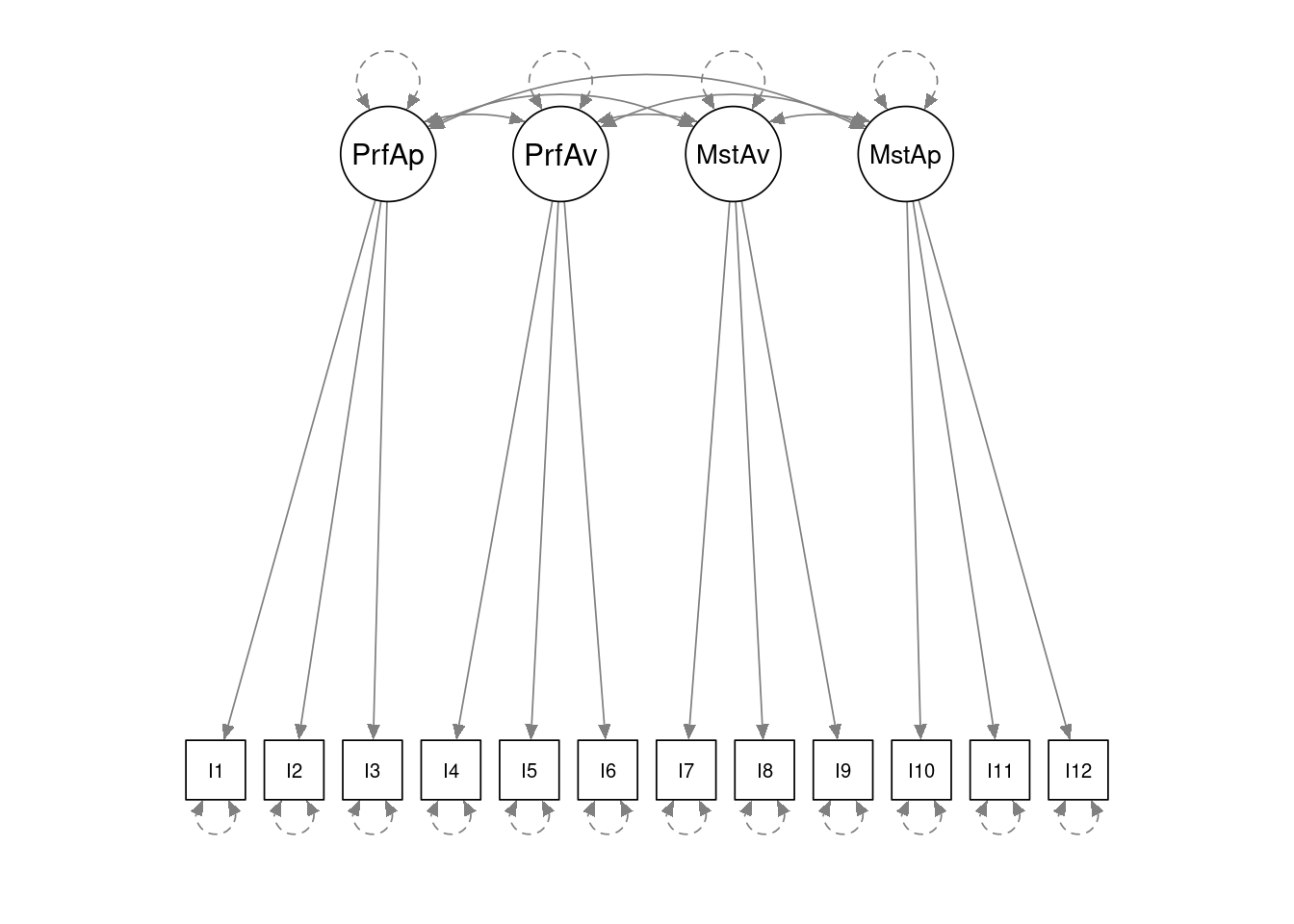
Model Estimation
Use the lavaan::cfa() function
- Use the first item as the reference indicator
# Default of lavaan::cfa
cfa_fit <- cfa(cfa_mod,
    sample.cov = covy,
    # number of observations
    sample.nobs = 1022,
    # default option to correlate latent factors
    auto.cov.lv.x = TRUE,
    # Model identified by fixing the loading of first indicator to 1
    std.lv = FALSE
)- Standardize latent variable
Technically speaking, this is still not fully identified, because the results will be the same with \(\symbf \Lambda* = -\symbf \Lambda\)
# Default of lavaan::cfa
cfa_fit2 <- cfa(cfa_mod,
    sample.cov = covy,
    # number of observations
    sample.nobs = 1022,
    # Model identified by standardizing the latent variables
    std.lv = TRUE
)
As can be seen below, the two ways of identification give the same implied covariance matrix, but the estimates are different because the latent variables are in different units.
# Implied covariance
lavInspect(cfa_fit, what = "cov.ov") -
    lavInspect(cfa_fit2, what = "cov.ov")
I1 I2 I3 I4 I5 I6 I7 I8 I9 I10 I11 I12
I1 0
I2 0 0
I3 0 0 0
I4 0 0 0 0
I5 0 0 0 0 0
I6 0 0 0 0 0 0
I7 0 0 0 0 0 0 0
I8 0 0 0 0 0 0 0 0
I9 0 0 0 0 0 0 0 0 0
I10 0 0 0 0 0 0 0 0 0 0
I11 0 0 0 0 0 0 0 0 0 0 0
I12 0 0 0 0 0 0 0 0 0 0 0 0msummary(
list(`reference indicator` = cfa_fit,
`standardized latent factor` = cfa_fit2))| reference indicator | standardized latent factor | |
|---|---|---|
| PerfAppr =~ I1 | 1.000 | 1.258 |
| (0.000) | (0.042) | |
| PerfAppr =~ I2 | 1.034 | 1.300 |
| (0.036) | (0.041) | |
| PerfAppr =~ I3 | 1.053 | 1.324 |
| (0.036) | (0.042) | |
| PerfAvoi =~ I4 | 1.000 | 1.145 |
| (0.000) | (0.064) | |
| PerfAvoi =~ I5 | 0.772 | 0.884 |
| (0.061) | (0.056) | |
| PerfAvoi =~ I6 | 1.197 | 1.370 |
| (0.081) | (0.057) | |
| MastAvoi =~ I7 | 1.000 | 0.655 |
| (0.000) | (0.046) | |
| MastAvoi =~ I8 | 1.955 | 1.281 |
| (0.149) | (0.047) | |
| MastAvoi =~ I9 | 1.856 | 1.216 |
| (0.139) | (0.051) | |
| MastAppr =~ I10 | 1.000 | 0.815 |
| (0.000) | (0.037) | |
| MastAppr =~ I11 | 0.974 | 0.794 |
| (0.052) | (0.030) | |
| MastAppr =~ I12 | 1.042 | 0.850 |
| (0.057) | (0.037) | |
| PerfAppr ~~ PerfAvoi | 0.752 | 0.522 |
| (0.074) | (0.032) | |
| PerfAppr ~~ MastAvoi | 0.196 | 0.238 |
| (0.034) | (0.035) | |
| PerfAppr ~~ MastAppr | 0.309 | 0.301 |
| (0.042) | (0.035) | |
| PerfAvoi ~~ MastAvoi | 0.377 | 0.503 |
| (0.046) | (0.034) | |
| PerfAvoi ~~ MastAppr | 0.080 | 0.086 |
| (0.039) | (0.041) | |
| MastAvoi ~~ MastAppr | 0.159 | 0.297 |
| (0.025) | (0.036) | |
| Num.Obs. | 1022 | 1022 |
| AIC | 40102.2 | 40102.2 |
| BIC | 40250.1 | 40250.1 |
Model Fit
summary(cfa_fit2, fit.measures = TRUE)lavaan 0.6.15 ended normally after 26 iterations
Estimator ML
Optimization method NLMINB
Number of model parameters 30
Number of observations 1022
Model Test User Model:
Test statistic 284.199
Degrees of freedom 48
P-value (Chi-square) 0.000
Model Test Baseline Model:
Test statistic 4419.736
Degrees of freedom 66
P-value 0.000
User Model versus Baseline Model:
Comparative Fit Index (CFI) 0.946
Tucker-Lewis Index (TLI) 0.925
Loglikelihood and Information Criteria:
Loglikelihood user model (H0) -20021.119
Loglikelihood unrestricted model (H1) -19879.019
Akaike (AIC) 40102.238
Bayesian (BIC) 40250.123
Sample-size adjusted Bayesian (SABIC) 40154.840
Root Mean Square Error of Approximation:
RMSEA 0.069
90 Percent confidence interval - lower 0.062
90 Percent confidence interval - upper 0.077
P-value H_0: RMSEA <= 0.050 0.000
P-value H_0: RMSEA >= 0.080 0.013
Standardized Root Mean Square Residual:
SRMR 0.050
Parameter Estimates:
Standard errors Standard
Information Expected
Information saturated (h1) model Structured
Latent Variables:
Estimate Std.Err z-value P(>|z|)
PerfAppr =~
I1 1.258 0.042 29.924 0.000
I2 1.300 0.041 31.911 0.000
I3 1.324 0.042 31.876 0.000
PerfAvoi =~
I4 1.145 0.064 17.768 0.000
I5 0.884 0.056 15.662 0.000
I6 1.370 0.057 24.048 0.000
MastAvoi =~
I7 0.655 0.046 14.109 0.000
I8 1.281 0.047 27.004 0.000
I9 1.216 0.051 23.855 0.000
MastAppr =~
I10 0.815 0.037 22.167 0.000
I11 0.794 0.030 26.297 0.000
I12 0.850 0.037 22.762 0.000
Covariances:
Estimate Std.Err z-value P(>|z|)
PerfAppr ~~
PerfAvoi 0.522 0.032 16.537 0.000
MastAvoi 0.238 0.035 6.737 0.000
MastAppr 0.301 0.035 8.672 0.000
PerfAvoi ~~
MastAvoi 0.503 0.034 14.794 0.000
MastAppr 0.086 0.041 2.094 0.036
MastAvoi ~~
MastAppr 0.297 0.036 8.164 0.000
Variances:
Estimate Std.Err z-value P(>|z|)
.I1 0.819 0.050 16.297 0.000
.I2 0.649 0.046 13.975 0.000
.I3 0.678 0.048 14.021 0.000
.I4 2.448 0.133 18.460 0.000
.I5 2.039 0.103 19.748 0.000
.I6 1.077 0.109 9.896 0.000
.I7 1.585 0.075 21.188 0.000
.I8 0.607 0.080 7.632 0.000
.I9 1.111 0.084 13.207 0.000
.I10 0.727 0.043 16.785 0.000
.I11 0.329 0.030 10.837 0.000
.I12 0.717 0.045 16.095 0.000
PerfAppr 1.000
PerfAvoi 1.000
MastAvoi 1.000
MastAppr 1.000 Residuals and Modification Indices
resid(cfa_fit2, type = "cor")$type
[1] "cor.bollen"
$cov
I1 I2 I3 I4 I5 I6 I7 I8 I9 I10
I1 0.000
I2 0.000 0.000
I3 0.013 -0.010 0.000
I4 -0.084 -0.017 -0.074 0.000
I5 -0.060 0.014 -0.055 0.069 0.000
I6 -0.045 0.067 0.062 0.011 -0.043 0.000
I7 -0.129 -0.026 -0.072 0.090 0.206 0.053 0.000
I8 -0.022 0.039 0.044 -0.036 0.054 -0.017 -0.008 0.000
I9 -0.068 -0.008 0.010 -0.105 0.054 -0.002 -0.014 0.005 0.000
I10 0.111 0.077 0.046 0.004 0.035 0.012 -0.077 -0.024 -0.026 0.000
I11 -0.016 -0.006 -0.022 -0.029 -0.045 -0.004 -0.059 -0.004 -0.005 -0.002
I12 -0.061 -0.027 -0.053 -0.007 -0.011 0.036 0.063 0.041 0.046 -0.007
I11 I12
I1
I2
I3
I4
I5
I6
I7
I8
I9
I10
I11 0.000
I12 0.006 0.000modindices(cfa_fit2, sort = TRUE, minimum = 10)Because the correlation residuals and modification indices suggest unmodelled correlations between Items 5 and 7, we can modify our model
cfa_modr <- "
    # Loadings
    PerfAppr =~ I1 + I2 + I3
    PerfAvoi =~ I4 + I5 + I6
    MastAvoi =~ I7 + I8 + I9
    MastAppr =~ I10 + I11 + I12
    # Factor covariances (can be omitted)
    PerfAppr ~~ PerfAvoi + MastAvoi + MastAppr
    PerfAvoi ~~ MastAvoi + MastAppr
    MastAvoi ~~ MastAppr
    # Unique covariances
    I5 ~~ I7
"
cfa_fitr <- cfa(cfa_modr,
    sample.cov = covy,
    sample.nobs = 1022,
    std.lv = TRUE
)
# Check residuals and modification indices again
resid(cfa_fitr, type = "cor")
$type
[1] "cor.bollen"
$cov
I1 I2 I3 I4 I5 I6 I7 I8 I9 I10
I1 0.000
I2 0.000 0.000
I3 0.012 -0.010 0.000
I4 -0.086 -0.019 -0.076 0.000
I5 -0.056 0.019 -0.050 0.083 0.000
I6 -0.052 0.060 0.055 0.014 -0.030 0.000
I7 -0.126 -0.022 -0.069 0.098 0.050 0.062 0.000
I8 -0.025 0.037 0.042 -0.032 0.063 -0.018 0.007 0.000
I9 -0.069 -0.009 0.009 -0.100 0.063 0.000 0.002 0.004 0.000
I10 0.111 0.077 0.046 0.003 0.035 0.010 -0.073 -0.025 -0.026 0.000
I11 -0.016 -0.006 -0.022 -0.030 -0.044 -0.006 -0.055 -0.006 -0.005 -0.002
I12 -0.061 -0.027 -0.053 -0.008 -0.011 0.034 0.067 0.040 0.046 -0.007
I11 I12
I1
I2
I3
I4
I5
I6
I7
I8
I9
I10
I11 0.000
I12 0.006 0.000modindices(cfa_fitr, sort = TRUE, minimum = 10)Composite Reliability
(omegas <- compRelSEM(cfa_fitr))PerfAppr PerfAvoi MastAvoi MastAppr
0.875 0.648 0.741 0.774 Reporting
Path Diagram
You can use the semPlot::semPaths() function for path diagrams with estimates. To make the plot a bit nicer, try the semptools package.
p <- semPaths(
    cfa_fitr,
    whatLabels = "est",
    nCharNodes = 0,
    sizeMan = 4,
    node.width = 1,
    edge.label.cex = .65,
    # Larger margin
    mar = c(8, 5, 12, 5),
    DoNotPlot = TRUE
)
p2 <- set_cfa_layout(
    p,
    indicator_order = paste0("I", 1:12),
    indicator_factor = rep(c("PerfAppr", "PerfAvoi",
                             "MastAvoi", "MastAppr"),
                           each = 3),
    # Make covariances more curved
    fcov_curve = 1.75,
    # Move loadings down
    loading_position = .8) |>
    mark_se(object = cfa_fitr, sep = "\n")
plot(p2)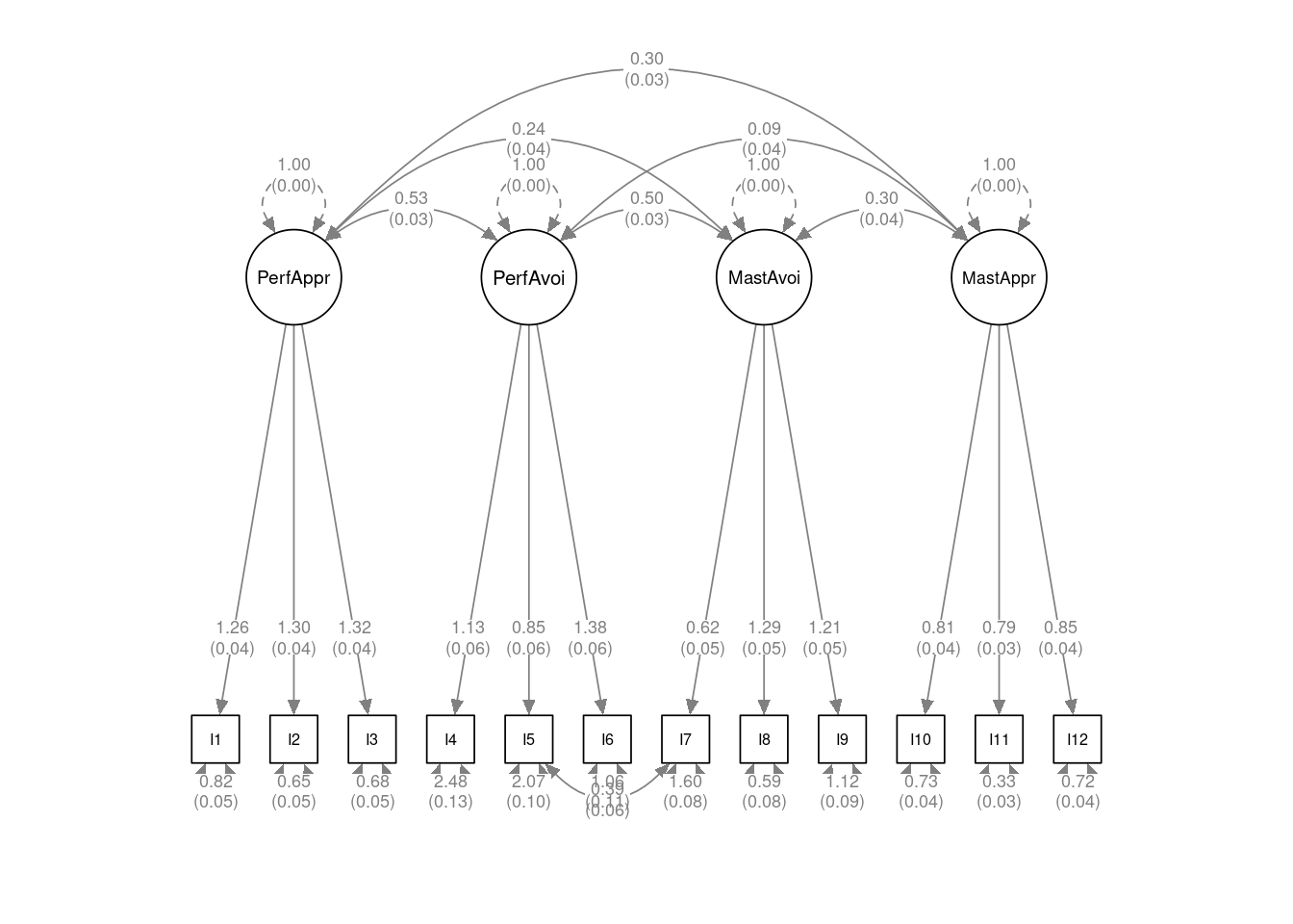
Table
# Extract estimates
parameterEstimates(cfa_fitr) |>
    # filter only loadings and variances
    dplyr::filter(grepl("^I.*", rhs)) |>
    # Remove unique covariance
    dplyr::filter(op == "=~" | lhs == rhs) |>
    # select columns
    dplyr::select(op, rhs, est, ci.lower, ci.upper) |>
    # make loadings and variances in different columns
    tidyr::pivot_wider(names_from = op,
                       values_from = 3:5) |>
    # add rows
    tibble::add_row(rhs = "Mastery Approach", .before = 10) |>
    tibble::add_row(rhs = "Mastery Avoidance", .before = 7) |>
    tibble::add_row(rhs = "Perform Avoidance", .before = 4) |>
    tibble::add_row(rhs = "Perform Approach", .before = 1) |>
    flextable::flextable() |>
    # Two digits
    colformat_double(digits = 2) |>
    # Set heading
    set_header_labels(
        values = c("item", "Est", "LL", "UL", "Est", "LL", "UL")
    ) |>
    add_header_row(
        values = c("", "Loading", "Uniqueness"),
        colwidths = c(1, 3, 3)
    ) |>
    # merge columns
    merge_h_range(i = c(1, 5, 9, 13), j1 = 1, j2 = 7) |>
    # alignment
    align(i = 1, align = "center", part = "header") |>
align(i = c(1, 5, 9, 13), align = "center", part = "body")Loading | Uniqueness | |||||
|---|---|---|---|---|---|---|
item | Est | LL | UL | Est | LL | UL |
Perform Approach | ||||||
I1 | 1.26 | 0.82 | 1.18 | 0.72 | 1.34 | 0.92 |
I2 | 1.30 | 0.65 | 1.22 | 0.56 | 1.38 | 0.74 |
I3 | 1.32 | 0.68 | 1.24 | 0.58 | 1.41 | 0.77 |
Perform Avoidance | ||||||
I4 | 1.13 | 2.48 | 1.01 | 2.21 | 1.26 | 2.74 |
I5 | 0.85 | 2.07 | 0.74 | 1.87 | 0.96 | 2.27 |
I6 | 1.38 | 1.06 | 1.26 | 0.84 | 1.49 | 1.28 |
Mastery Avoidance | ||||||
I7 | 0.62 | 1.60 | 0.53 | 1.45 | 0.71 | 1.75 |
I8 | 1.29 | 0.59 | 1.19 | 0.43 | 1.38 | 0.75 |
I9 | 1.21 | 1.12 | 1.11 | 0.95 | 1.31 | 1.29 |
Mastery Approach | ||||||
I10 | 0.81 | 0.73 | 0.74 | 0.64 | 0.89 | 0.81 |
I11 | 0.79 | 0.33 | 0.73 | 0.27 | 0.85 | 0.39 |
I12 | 0.85 | 0.72 | 0.78 | 0.63 | 0.92 | 0.80 |
# Latent correlations
cor_lv <- lavInspect(cfa_fitr, what = "cor.lv")
# Remove upper part
cor_lv[upper.tri(cor_lv, diag = TRUE)] <- NA
cor_lv |>
    as.data.frame() |>
    rownames_to_column("var") |>
    # Number first column
    mutate(var = paste0(1:4, ".", var)) |>
    flextable::flextable() |>
    colformat_double(digits = 2) |>
    set_header_labels(
        values = c("", "1", "2", "3", "4")
)1 | 2 | 3 | 4 | |
|---|---|---|---|---|
1.PerfAppr | ||||
2.PerfAvoi | 0.53 | |||
3.MastAvoi | 0.24 | 0.50 | ||
4.MastAppr | 0.30 | 0.09 | 0.30 |
We fit a 4-factor model with each item loading on one of the four factors: Performance Approach (Items 1 to 3), Performance Avoidance (Items 4 to 6), Mastery Avoidance (Items 7 to 9), and Mastery Approach (Items 10 to 12). We used the lavaan package (v0.6.15; Rosseel, 2012) with normal distribution-based maximum likelihood estimation. There were no missing data as all participants responded to all items. We evaluate the model using the global \(\chi^2\) test, as well as goodness-of-fit indices including RMSEA (≤ .05 indicating good fit; Browne & Cudeck, 1993), CFI (≥ .95 indicating good fit; Hu & Bentler, 1999), and SRMR (≤ .08 indicating acceptable fit; Hu & Bentler, 1999). We also consider the correlation residuals and the modification indices.
The \(\chi^2\) test indicated that the hypothesized 4-factor model does not perfectly fit the data, \(\chi^2\)(N = 1022, df = 48) = 284, p < .001. However, the fit is reasonable, with RMSEA = .07, 90% CI [.06, .08], CFI = .95, and SRMR = .05. Inspection of the correlation residuals shows relatively large unmodelled correlations between Items 5 and 7 (0.21), and modification indices similarly suggest adding unique covariance between those two items (MI = 40.3961327).
Given that the two items have similar wordings, we refit the model with unique covariance between them. The model fit improves, \(\chi^2\)(N = 1022, df = 47) = 242, p < .001, RMSEA = .06, 90% CI [.06, .07], CFI = .96, and SRMR = .04. Further inspection of correlation residuals and modification indices does not suggest modifications to the model that are theoretically justified.
Figure 1, Table 1, and Table 2 show the parameter estimates of the loadings and uniqueness, based on the final model. When forming composites for the four latent factors, the omega coefficient for the composite reliability is .87 for Performance Approach, .65 for Performance Avoidance, .74 for Mastery Avoidance (Items 7 to 9), and .77 for Mastery Approach.
Example 2: Non-normal Data
Note that methods such MLR and WLSMV require the input of either (a) the raw data or (b) an asymptotic covariance matrix for the sample covariances. We’ll use the bfi data set as an example here.
ac_mod <- "
Ag =~ A1 + A2 + A3 + A4 + A5
Co =~ C1 + C2 + C3 + C4 + C5
"
# MLR
cfa_ac_mlr <- cfa(
    ac_mod,
    data = bfi,
    missing = "fiml",
    estimator = "MLR",
    std.lv = TRUE
)
# WLSMV (missing data with listwise)
cfa_ac_wls <- cfa(
    ac_mod,
    data = bfi,
    ordered = TRUE,
    estimator = "WLSMV",  # default when `ordered = TRUE`
    std.lv = TRUE
)
# Compare
msummary(
    list(MLR = cfa_ac_mlr, WLSMV = cfa_ac_wls),
    shape = term ~ model + statistic
)| Est. | S.E. | Est. | S.E. | |
|---|---|---|---|---|
| Ag =~ A1 | 0.520 | 0.033 | 0.408 | 0.019 |
| Ag =~ A2 | −0.775 | 0.027 | −0.722 | 0.013 |
| Ag =~ A3 | −0.973 | 0.029 | −0.787 | 0.012 |
| Ag =~ A4 | −0.733 | 0.032 | −0.570 | 0.017 |
| Ag =~ A5 | −0.791 | 0.027 | −0.676 | 0.014 |
| Co =~ C1 | 0.668 | 0.032 | 0.595 | 0.016 |
| Co =~ C2 | 0.801 | 0.032 | 0.664 | 0.014 |
| Co =~ C3 | 0.715 | 0.028 | 0.593 | 0.015 |
| Co =~ C4 | −0.915 | 0.030 | −0.722 | 0.014 |
| Co =~ C5 | −0.965 | 0.035 | −0.644 | 0.014 |
| Ag ~~ Co | −0.341 | 0.028 | −0.371 | 0.022 |
| Num.Obs. | 2800 | 2632 | ||
| AIC | 90191.5 | |||
| BIC | 90375.6 |
# Fit indices
summary(
    semTools::compareFit(cfa_ac_mlr, cfa_ac_wls, nested = FALSE)
)
Warning in semTools::compareFit(cfa_ac_mlr, cfa_ac_wls, nested = FALSE):
fitMeasures() returned vectors of different lengths for different models,
probably because certain options are not the same. Check lavInspect(fit,
"options")[c("estimator","test","meanstructure")] for each model, or run
fitMeasures() on each model to investigate.####################### Model Fit Indices ###########################
chisq.scaled df.scaled pvalue.scaled rmsea.robust cfi.robust
cfa_ac_mlr 466.460† 34 .000 .073† .910†
cfa_ac_wls 593.496 34 .000 .087 .905
tli.robust srmr
cfa_ac_mlr .880† .043†
cfa_ac_wls .875 .051 Weight Matrix (Asymptotic Covariance Matrix of the Sample Covariance Matrix)
[This and the remainder contains more mathematical details.]
Estimators like MLM, MLR, and WLSMV make use of the asymptotic covariance matrix, which is called NACOV or gamma in lavaan. This is an estimated covariance matrix for the sample statistics, and is generally huge in size. For example, if the input matrix is 10 × 10, there are 55 unique variances/covariances, so the asymptotic matrix is 55 × 55.
# Refit with listwise deletion and MLM so that
# we don't worry about missing data here
cfa_ac_mlm <- cfa(
    ac_mod,
    data = bfi,
    estimator = "MLM"
)
ac_gamma_mlm <- lavInspect(cfa_ac_mlm, what = "gamma")
dim(ac_gamma_mlm)
[1] 55 55Each element of the matrix is a covariance of the covariance. First, note that the covariance is
\[\sigma_{XY} = E\{[X - E(Y)] \times [Y - E(Y)]\}\]
The covariance of the covariance is
\[\sigma_{ABCD} = E\{[A - E(A)] \times [B - E(B)] \times [C - E(C)] \times [D - E(D)]\} - \sigma_{AB} \sigma_{CD}\]
dat <- lavInspect(cfa_ac_mlm, what = "data")
# First, center the data
dat_c <- scale(dat, center = TRUE, scale = FALSE)
# For example, covariance of (a) cov(A1, A2) and (b) cov(A3, A4)
mean(dat_c[, 1] * dat_c[, 2] * dat_c[, 3] * dat_c[, 4]) -
    cov(dat_c[, 1], dat_c[, 2]) * cov(dat_c[, 3], dat_c[, 4])
[1] -0.7339502ac_gamma_mlm["A1~~A2", "A3~~A4"][1] -0.7342573The two values almost match, except that in lavaan, the covariance is computed by dividing by \(N\) (instead of \(N - 1\) as in cov). The following computes the asymptotic covariance matrix:
N <- nobs(cfa_ac_mlm)
# Sample covariance S (uncorrected)
Sy <- cov(dat) * (N - 1) / N
# Centered data, and transpose
ac_gamma_hand <- tcrossprod(
    apply(dat_c, 1, tcrossprod) - as.vector(Sy)
) / N
# Remove duplicated elements
unique_Sy <- as.vector(lower.tri(Sy, diag = TRUE))
# Check the matrices are the same
all.equal(ac_gamma_hand[unique_Sy, unique_Sy],
          unname(unclass(ac_gamma_mlm)))
[1] TRUE# MLM using the sample covariance matrix and the asymptotic covariance matrix
cfa(ac_mod,
sample.cov = cov(dat),
sample.nobs = N,
estimator = "MLM",
NACOV = ac_gamma_hand[unique_Sy, unique_Sy]
)lavaan 0.6.15 ended normally after 40 iterations
Estimator ML
Optimization method NLMINB
Number of model parameters 21
Number of observations 2632
Model Test User Model:
Standard Scaled
Test Statistic 503.340 424.760
Degrees of freedom 34 34
P-value (Chi-square) 0.000 0.000
Scaling correction factor 1.185
Satorra-Bentler correction Mathematical and Computational Details
\[ \DeclareMathOperator{\Tr}{tr} \DeclareMathOperator{\vech}{vech} \]
Discrepancy function for Normal-Distribution ML
Let \(\boldsymbol{\eta} = [\eta_1, \ldots, \eta_q]^\top\) be the latent factors. Without loss of generality, assume that the items are mean-centered. Assume normality, our factor model becomes
\[ \begin{aligned} \symbf y | \boldsymbol \eta_q & \sim N_p(\symbf{\Lambda} \boldsymbol \eta_q, \symbf \Theta) \\ \boldsymbol \eta_q & \sim N_p(\symbf 0, \symbf \Theta) \end{aligned}, \]
which implies that the marginal distribution of \(\symbf y\) is also normal:
\[ \symbf y \sim N_p(\symbf 0, \symbf\Sigma) \]
The log-density of \(\symbf y_i\) for person \(i\), which is multivariate normal of dimension \(p\), is
\[ \log f(\symbf y_i; \symbf\Sigma) = -\frac{1}{2} \log(2 \pi) - \frac{1}{2} \log |\symbf \Sigma| - \frac{1}{2} \symbf y_i^\top \symbf \Sigma^{-1} \symbf y_i \]
The quadratic form \(\symbf y_i^\top \symbf \Sigma^{-1} \symbf y_i\) can be written as \(\Tr(\symbf y_i^\top \symbf \Sigma^{-1} \symbf y_i)\) = \(\Tr(\symbf \Sigma^{-1} \symbf y_i \symbf y_i^\top)\), which uses a property of the matrix trace.
Specified model (H0)
The log-likelihood of the data, assuming that each participant is independent, is
\[ \begin{aligned} \ell(\symbf\Sigma; \symbf y_i, \ldots, \symbf y_N) & = - \frac{Np}{2} \log(2\pi) - \frac{N}{2} \log |\symbf \Sigma| - \frac{1}{2} \sum_i^N \Tr \left(\symbf \Sigma^{-1} \symbf y_i \symbf y_i^\top\right) \\ & = - \frac{Np}{2} \log(2\pi) - \frac{N}{2} \log |\symbf \Sigma| - \frac{1}{2} \Tr\left(\symbf \Sigma^{-1} \sum_i^N \symbf y_i \symbf y_i^\top\right) \end{aligned} \]
Because \(\sum_i^N \symbf y_i \symbf y_i^\top\), the sum of cross-products, is \((N - 1) \symbf S\) where \(\symbf S\) is the sample covariance matrix (you should verify this yourself), we can see \(\symbf S\) is sufficient for inference, and
\[ \ell(\symbf\Sigma; \symbf S) = - \frac{Np}{2} \log(2\pi) - \frac{N}{2} \log |\symbf \Sigma| - \frac{N - 1}{2} \Tr \left(\symbf \Sigma^{-1} \symbf S\right) \]
You can verify this in lavaan
# Implied covariance
sigmahat_mat <- lavInspect(cfa_fit, what = "cov.ov")
ny <- 1022
py <- 12 # number of items
logdet_sigma <- as.vector(determinant(sigmahat_mat, log = TRUE)$modulus)
ll <- -ny * py / 2 * log(2 * pi) - ny / 2 * logdet_sigma -
    (ny - 1) / 2 * sum(diag(solve(sigmahat_mat, covy)))
print(ll)
[1] -20021.12# Compare to lavaan
logLik(cfa_fit)'log Lik.' -20021.12 (df=30)Here is a code example for finding MLE of the above model in R:
# 1. Define a function that converts a parameter vector
#    to the implied covariances
implied_cov <- function(pars) {
    # Initialize Lambda (first indicator fixed to 1)
    lambda_mat <- matrix(0, nrow = 12, ncol = 4)
    lambda_mat[1, 1] <- 1
    lambda_mat[4, 2] <- 1
    lambda_mat[7, 3] <- 1
    lambda_mat[10, 4] <- 1
    # Fill the first eight values of pars to the matrix
    lambda_mat[2:3, 1] <- pars[1:2]
    lambda_mat[5:6, 2] <- pars[3:4]
    lambda_mat[8:9, 3] <- pars[5:6]
    lambda_mat[11:12, 4] <- pars[7:8]
    # Fill the next 10 values to the Psi matrix
    psi_mat <- getCov(pars[9:18])
    # Fill the Theta matrix
    theta_mat <- diag(pars[19:30])
    # Implied covariances
    lambda_mat %*% tcrossprod(psi_mat, lambda_mat) + theta_mat
}
# 2. Set initial values
pars0 <- c(
    # loadings
    rep(1, 8),
    # psi
    1,
    .3, 1,
    .3, .3, 1,
    .3, .3, .3, 1,
    # theta
    rep(1, 12)
)
# 3. Likelihood function
fitfunction_ml <- function(pars, covy, ny = 1022) {
    py <- nrow(covy)
    sigmahat_mat <- implied_cov(pars)
    logdet_sigma <- as.vector(determinant(sigmahat_mat, log = TRUE)$modulus)
    -ny * py / 2 * log(2 * pi) - ny / 2 * logdet_sigma -
        (ny - 1) / 2 * sum(diag(solve(sigmahat_mat, covy)))
}
# fitfunction_ml(pars0, covy)
# 4. Optimization
opt <- optim(pars0,
             fn = fitfunction_ml,
             covy = covy,
             method = "L-BFGS-B",
             # Minimize -2 x ll
             control = list(fnscale = -2))
# 5. Results
opt$par[1:8]  # Lambda
[1] 1.0335938 1.0530526 0.7713447 1.1950028 1.9569734 1.8569790 0.9742877
[8] 1.0423243# Compare to lavaan
lavInspect(cfa_fit, what = "est")$lambda PrfApp PerfAv MastAv MstApp
I1 1.000 0.000 0.000 0.000
I2 1.034 0.000 0.000 0.000
I3 1.053 0.000 0.000 0.000
I4 0.000 1.000 0.000 0.000
I5 0.000 0.772 0.000 0.000
I6 0.000 1.197 0.000 0.000
I7 0.000 0.000 1.000 0.000
I8 0.000 0.000 1.955 0.000
I9 0.000 0.000 1.856 0.000
I10 0.000 0.000 0.000 1.000
I11 0.000 0.000 0.000 0.974
I12 0.000 0.000 0.000 1.042getCov(opt$par[9:18],
names = paste0("F", 1:4)) # Psi F1 F2 F3 F4
F1 1.5812970 0.7532855 0.1963523 0.3088340
F2 0.7532855 1.3144956 0.3773226 0.0801237
F3 0.1963523 0.3773226 0.4286353 0.1586037
F4 0.3088340 0.0801237 0.1586037 0.6642753# Compare to lavaan
lavInspect(cfa_fit, what = "est")$psi PrfApp PerfAv MastAv MstApp
PerfAppr 1.582
PerfAvoi 0.752 1.312
MastAvoi 0.196 0.377 0.429
MastAppr 0.309 0.080 0.159 0.664diag(opt$par[19:30]) # Theta [,1] [,2] [,3] [,4] [,5] [,6] [,7]
[1,] 0.818593 0.0000000 0.0000000 0.000000 0.000000 0.000000 0.000000
[2,] 0.000000 0.6491388 0.0000000 0.000000 0.000000 0.000000 0.000000
[3,] 0.000000 0.0000000 0.6775787 0.000000 0.000000 0.000000 0.000000
[4,] 0.000000 0.0000000 0.0000000 2.446722 0.000000 0.000000 0.000000
[5,] 0.000000 0.0000000 0.0000000 0.000000 2.037345 0.000000 0.000000
[6,] 0.000000 0.0000000 0.0000000 0.000000 0.000000 1.078629 0.000000
[7,] 0.000000 0.0000000 0.0000000 0.000000 0.000000 0.000000 1.585625
[8,] 0.000000 0.0000000 0.0000000 0.000000 0.000000 0.000000 0.000000
[9,] 0.000000 0.0000000 0.0000000 0.000000 0.000000 0.000000 0.000000
[10,] 0.000000 0.0000000 0.0000000 0.000000 0.000000 0.000000 0.000000
[11,] 0.000000 0.0000000 0.0000000 0.000000 0.000000 0.000000 0.000000
[12,] 0.000000 0.0000000 0.0000000 0.000000 0.000000 0.000000 0.000000
[,8] [,9] [,10] [,11] [,12]
[1,] 0.0000000 0.00000 0.0000000 0.0000000 0.0000000
[2,] 0.0000000 0.00000 0.0000000 0.0000000 0.0000000
[3,] 0.0000000 0.00000 0.0000000 0.0000000 0.0000000
[4,] 0.0000000 0.00000 0.0000000 0.0000000 0.0000000
[5,] 0.0000000 0.00000 0.0000000 0.0000000 0.0000000
[6,] 0.0000000 0.00000 0.0000000 0.0000000 0.0000000
[7,] 0.0000000 0.00000 0.0000000 0.0000000 0.0000000
[8,] 0.6062578 0.00000 0.0000000 0.0000000 0.0000000
[9,] 0.0000000 1.11147 0.0000000 0.0000000 0.0000000
[10,] 0.0000000 0.00000 0.7266675 0.0000000 0.0000000
[11,] 0.0000000 0.00000 0.0000000 0.3288637 0.0000000
[12,] 0.0000000 0.00000 0.0000000 0.0000000 0.7168119lavInspect(cfa_fit, what = "est")$theta I1 I2 I3 I4 I5 I6 I7 I8 I9 I10 I11 I12
I1 0.819
I2 0.000 0.649
I3 0.000 0.000 0.678
I4 0.000 0.000 0.000 2.448
I5 0.000 0.000 0.000 0.000 2.039
I6 0.000 0.000 0.000 0.000 0.000 1.077
I7 0.000 0.000 0.000 0.000 0.000 0.000 1.585
I8 0.000 0.000 0.000 0.000 0.000 0.000 0.000 0.607
I9 0.000 0.000 0.000 0.000 0.000 0.000 0.000 0.000 1.111
I10 0.000 0.000 0.000 0.000 0.000 0.000 0.000 0.000 0.000 0.727
I11 0.000 0.000 0.000 0.000 0.000 0.000 0.000 0.000 0.000 0.000 0.329
I12 0.000 0.000 0.000 0.000 0.000 0.000 0.000 0.000 0.000 0.000 0.000 0.717# 6. Maximized log-likelihood
opt$value[1] -20021.12Saturated model (H1)
In a saturated model, it can be shown that \(\hat{\symbf\Sigma} = \tilde{\symbf S} = (N - 1) \symbf S / N\) such that the model-implied covariance matrix is the same as the sample covariance matrix. Thus, \(\Tr (\hat{\symbf \Sigma}^{-1} \symbf S)\) = \(N \Tr (\symbf I) / (N - 1)\) = \(Np / (N - 1)\), and the saturated loglikelihood is
\[ \ell_1 = \ell(\symbf \Sigma = \symbf S; \symbf S) = - \frac{Np}{2} (\log(2\pi) + 1) - \frac{N}{2} \log |\tilde{\symbf S}| - \frac{Np}{2} \]
tilde_s <- (ny - 1) / ny * covy
logdet_tilde_s <- as.vector(determinant(tilde_s, log = TRUE)$modulus)
ll1 <- -ny * py / 2 * log(2 * pi) - ny / 2 * logdet_tilde_s -
    ny * py / 2
print(ll1)
[1] -19879.02Likelihood-ratio test statistic (\(\chi^2\))
\[ \begin{aligned} T = -2 [\ell(\hat{\symbf\Sigma}; \symbf S) - \ell_1] & = N \left[\log |\hat{\symbf \Sigma}| - \log |\tilde{\symbf S}| + \Tr \left(\hat{\symbf \Sigma}^{-1}\tilde{\symbf S}\right) - p\right] \end{aligned} \]
ny * (logdet_sigma - logdet_tilde_s +
    sum(diag(solve(sigmahat_mat, tilde_s))) - py)
[1] 284.1989# Compared to the results in lavaan
cfa_fit@test$standard$stat[1] 284.1989In a large sample, \(T\) follows a \(\chi^2\) distribution with degrees of freedom equals \(p (p + 1) / 2 - m\), where \(m\) is the number of parameters in the model.
Maximum likelihood can be used for categorical items, by using a model that treats the data as discrete instead of continuous. The computation is more intensive as the marginal distribution is no longer normal, and involves integrals that usually do not have close-form solutions.
Weighted Least Squares (WLS)
For continuous variables. The vech() operator converts the lower-diagonal elements of the covariance matrix into a vector.
\[ \begin{aligned} \symbf \sigma & = \vech(\symbf \Sigma) \\ \symbf s & = \vech(\symbf S) \end{aligned} \]
For our example, \(\vech(\Sigma)\) will have \(p (p + 1) / 2\) elements.
lavaan::lav_matrix_vech(covy) [1] 2.4025000 1.6363350 1.6974360 0.4991620 0.4244520 0.7811380
[7] -0.0880400 0.3324750 0.1946490 0.5121200 0.2764580 0.2083200
[13] 2.3409000 1.6994016 0.7272090 0.6374592 1.1079036 0.1477368
[19] 0.4865400 0.3571785 0.4585716 0.3028788 0.2827440 2.4336000
[25] 0.5689632 0.4691232 1.1162112 0.0465192 0.5077800 0.4093908
[31] 0.4104984 0.2843568 0.2396160 3.7636000 1.2384960 1.6083376
[37] 0.6253396 0.6343800 0.3716846 0.0892788 0.0228144 0.0675120
[43] 2.8224000 1.0893792 0.7824768 0.7056000 0.6870192 0.1308384
[49] -0.0131712 0.0423360 2.9584000 0.5812912 0.8385000 0.8335292
[55] 0.1197464 0.0859656 0.1733760 2.0164000 0.8221800 0.7658770
[61] 0.0301608 0.0723632 0.2726400 2.2500000 1.5721650 0.2690400
[67] 0.2969400 0.3978000 2.5921000 0.2450742 0.2792706 0.3960600
[73] 1.3924000 0.6452712 0.6839280 0.9604000 0.6820800 1.4400000# Same as
covy[lower.tri(covy, diag = TRUE)] [1] 2.4025000 1.6363350 1.6974360 0.4991620 0.4244520 0.7811380
[7] -0.0880400 0.3324750 0.1946490 0.5121200 0.2764580 0.2083200
[13] 2.3409000 1.6994016 0.7272090 0.6374592 1.1079036 0.1477368
[19] 0.4865400 0.3571785 0.4585716 0.3028788 0.2827440 2.4336000
[25] 0.5689632 0.4691232 1.1162112 0.0465192 0.5077800 0.4093908
[31] 0.4104984 0.2843568 0.2396160 3.7636000 1.2384960 1.6083376
[37] 0.6253396 0.6343800 0.3716846 0.0892788 0.0228144 0.0675120
[43] 2.8224000 1.0893792 0.7824768 0.7056000 0.6870192 0.1308384
[49] -0.0131712 0.0423360 2.9584000 0.5812912 0.8385000 0.8335292
[55] 0.1197464 0.0859656 0.1733760 2.0164000 0.8221800 0.7658770
[61] 0.0301608 0.0723632 0.2726400 2.2500000 1.5721650 0.2690400
[67] 0.2969400 0.3978000 2.5921000 0.2450742 0.2792706 0.3960600
[73] 1.3924000 0.6452712 0.6839280 0.9604000 0.6820800 1.4400000WLS finds a solution that minimizes
\[(\symbf s - \boldsymbol \sigma)^\top \symbf W^{-1} (\symbf s - \boldsymbol \sigma)\]
for some chosen weight matrix \(\symbf W\), which has dimension of \(p (p + 1) / 2 \times p (p + 1) / 2\).
For example, ULS uses an identity matrix as \(\symbf W\), so the above expression reduces to
\[(\symbf s - \boldsymbol \sigma)^\top (\symbf s - \boldsymbol \sigma)\]
Below is an example
uls_fit <- cfa(cfa_mod, sample.cov = covy,
               # number of observations
               sample.nobs = 1022,
               estimator = "ULS")
# Implied covariance matrix
sigmahat_uls <- lavInspect(uls_fit, what = "cov.ov")
# ULS discrepancy function
sum((sigmahat_uls - covy)^2) / 2
[1] 0.9677648# Verify that the ML solution gives a larger discrepancy
# based on the ULS criterion
sum((sigmahat_mat - covy)^2) / 2[1] 1.11625WLS is more commonly used as a fast alternative to maximum likelihood for categorical items. In such a situation, \(\symbf S\) and \(\symbf \Sigma\) are sample and model-implied polychoric correlation matrices, and the weight matrix is estimated based on the fourth moments (which is related to kurtosis) of the items. Taking the inverse of the full matrix, however, is very computationally intensive and unstable, as the matrix is huge (e.g., 78 \(\times\) 78) in our sample. Therefore, most applications use DWLS, the diagonally weighted version of it, where \(\symbf W\) is chosen as a diagonal matrix with the diagonal elements coming from the full matrix.
Here is a blog post I wrote about WLS: https://quantscience.rbind.io/2020/06/12/weighted-least-squares/