library(here)library(haven) # for reading SPSS datalibrary(tidyverse)library(lme4)
Warning in check_dep_version(): ABI version mismatch:
lme4 was built with Matrix ABI version 2
Current Matrix ABI version is 1
Please re-install lme4 from source or restore original 'Matrix' package
The file you need is the SPSS zip file from Chapter 10.
# Import data# Assume you downloaded the data to the folder "data", with the name# "Bandalos_Ch10_SPSS.zip"zip_data <-here("data", "Bandalos_Ch10_SPSS.zip")if (!file.exists(zip_data)) {dir.create("data")download.file("https://www.guilford.com/add/bandalos/Bandalos_Ch10_SPSS.zip", zip_data )}sample_data <-read_sav(unz( zip_data,"Bandalos_Ch10_SPSS/Data/Table 10.4 data untransposed.sav" ))sample_data
Data Transformation
While it’s possible to run analyses using the wide format, for our analyses we’ll transform the data to a long format as it better suits the analytic framework (variance components model) we’ll use. This also has better handling for missing data.
We’ll use the pivot_longer() function from the tidyr package (which is loaded with library(tidyverse)).
sample_long <-pivot_longer( sample_data,# select all columns, except the 1st one to be transformedcols =-1,# The columns have a pattern "R(1)Task(2)", where values# in parentheses are the IDs for the facets. So we first# specify this pattern, with a "." meaning a one-digit# place holder,names_pattern ="R(.)Task(.)",# and then specify that the first place holder is for rater,# and the second place-holder is for task.names_to =c("rater", "task"),values_to ="score"# name of score variable)head(sample_long)
As can be seen, the data are now in a long format.
Crossed Design
The data here has each participant (p) rated by the same three raters (r) on each of the three tasks (t). Therefore, this is a p\(\times\)r\(\times\)t design, where the two facets are crossed. We can see this by looking at the following tables:
With a crossed (factorial) design, every cell should be filled.
Contrast to Nested Design
On the other hand, if we have different sets of raters for different tasks, we will have a nested design. Let’s say we actually have 9 raters, with raters 1-3 for task 1, raters 4-6 for task 2, and raters 7-9 for task 3. This yields a p\(\times\) (r:t) design with raters nested within tasks.
When facet A is nested in facet B (i.e., a:b), each level of A is associated with only one level of B, but each level of B is associated with multiple levels of A.
# Variance components (VCs)vc_m1 <-as.data.frame(VarCorr(m1))# Organize in a table, similar to Table 10.4data.frame(source = vc_m1$grp,var = vc_m1$vcov,percent = vc_m1$vcov /sum(vc_m1$vcov))
Bootstrap Standard Errors and Confidence Intervals
get_vc <-function(x) { vc_x <-as.data.frame(VarCorr(x))c(vc_x$vcov, vc_x$vcov /sum(vc_x$vcov))}boo <-bootMer(m1, FUN = get_vc, nsim =1999)# Get percentile CIs for person varianceboot::boot.ci(boo, type ="perc", index =3)
BOOTSTRAP CONFIDENCE INTERVAL CALCULATIONS
Based on 1999 bootstrap replicates

CALL :
boot::boot.ci(boot.out = boo, type = "perc", index = 3)

Intervals :
Level     Percentile
95%   ( 0.171,  2.364 )
Calculations and Intervals on Original Scale
# Get percentile CIs for proportion of person varianceboot::boot.ci(boo, type ="perc", index =10)
BOOTSTRAP CONFIDENCE INTERVAL CALCULATIONS
Based on 1999 bootstrap replicates

CALL :
boot::boot.ci(boot.out = boo, type = "perc", index = 10)

Intervals :
Level     Percentile
95%   ( 0.1107,  0.6659 )
Calculations and Intervals on Original Scale
# Get percentile CIs for all VCsci_vc <-lapply(1:14, FUN =function(i) { ci_i <- boot::boot.ci(boo, type ="perc", index = i)$percentc(ll_var = ci_i[4], ul_var = ci_i[5])})
It also helps to create a function so that we can do the same operation in the future:
As shown above, while universe score variance (person variance) is the largest, it only accounts for a proportion of 0.4431584 of the total variance. If we use teminology analogous to classical test theory, it means that if we use a single rating of a single task to generalize to the universe score, less than half of the observed score variance is due to true score variance.
Interpreting the Variance Components
Venn diagrams
Venn diagram for variance components
Venn diagram closer to the actual example
Standard deviation
E.g., The ratings are on a 6-point scale. With \(\hat \sigma_{pr}\) = 0.6841528, this is the margin of error due to rater-by-person interaction, which is not trivial.
Treating Task as Fixed
# If treating task as fixed, the person x task variance will be averaged # and become part of the universe scorevaru <- vc_m1$vcov[3] + vc_m1$vcov[1] /3# The rater x task variance will be averaged and become part of rater variancevarr <- vc_m1$vcov[6] + vc_m1$vcov[4] /3# The residual will be averaged and become part of person x rater variancevare <- vc_m1$vcov[2] + vc_m1$vcov[7] /3# Combinedata.frame(source = vc_m1$grp[c(3, 6, 2)],var =c(varu, varr, vare),percent =c(varu, varr, vare) /sum(varu, varr, vare))
---title: "Generalizability Theory (Example 2)"format: html---```{r}#| echo: false# Define a function for formatting numberscomma <-function(x, d =2) format(x, digits = d, big.mark =",")``````{r}#| message: falselibrary(here)library(haven) # for reading SPSS datalibrary(tidyverse)library(lme4)```This second example comes from the companion website of the textbook, which can be downloaded here: <https://www.guilford.com/companion-site/Measurement-Theory-and-Applications-for-the-Social-Sciences/9781462532131>The file you need is the SPSS zip file from Chapter 10.```{r}# Import data# Assume you downloaded the data to the folder "data", with the name# "Bandalos_Ch10_SPSS.zip"zip_data <-here("data", "Bandalos_Ch10_SPSS.zip")if (!file.exists(zip_data)) {dir.create("data")download.file("https://www.guilford.com/add/bandalos/Bandalos_Ch10_SPSS.zip", zip_data )}sample_data <-read_sav(unz( zip_data,"Bandalos_Ch10_SPSS/Data/Table 10.4 data untransposed.sav" ))sample_data```## Data TransformationWhile it's possible to run analyses using the wide format, for our analyses we'll transform the data to a long format as it better suits the analytic framework (variance components model) we'll use. This also has better handling for missing data.We'll use the `pivot_longer()` function from the `tidyr` package (which is loaded with `library(tidyverse)`).```{r}sample_long <-pivot_longer( sample_data,# select all columns, except the 1st one to be transformedcols =-1,# The columns have a pattern "R(1)Task(2)", where values# in parentheses are the IDs for the facets. So we first# specify this pattern, with a "." meaning a one-digit# place holder,names_pattern ="R(.)Task(.)",# and then specify that the first place holder is for rater,# and the second place-holder is for task.names_to =c("rater", "task"),values_to ="score"# name of score variable)head(sample_long)```As can be seen, the data are now in a *long format*.## Crossed DesignThe data here has each participant (*p*) rated by the same three raters (*r*) on each of the three tasks (*t*). Therefore, this is a *p* $\times$ *r* $\times$ *t* design, where the two facets are crossed. We can see this by looking at the following tables:```{r}with(sample_long,table(person, rater))with(sample_long,table(rater, task))with(sample_long,table(person, task))```::: {.callout-note appearance="simple"}With a crossed (factorial) design, every cell should be filled. :::### Contrast to Nested DesignOn the other hand, if we have different sets of raters for different tasks, we will have a nested design. Let's say we actually have 9 raters, with raters 1-3 for task 1, raters 4-6 for task 2, and raters 7-9 for task 3. This yields a *p* $\times$ (*r*:*t*) design with raters nested within tasks.```{r}# Recode raterssample2 <- sample_long |>group_by(person) |>mutate(actual_rater =1:9) |>ungroup()with(sample2,table(person, actual_rater))with(sample2,table(actual_rater, task))with(sample2,table(person, task))```::: {.callout-note appearance="simple"}When facet A is nested in facet B (i.e., *a*:*b*), each level of A is associated with only one level of B, but each level of B is associated with multiple levels of A.:::## Variance Decomposition```{r}m1 <-lmer( score ~1+ (1| person) + (1| rater) + (1| task) + (1| person:rater) + (1| person:task) + (1| rater:task),data = sample_long)# Variance components (VCs)vc_m1 <-as.data.frame(VarCorr(m1))# Organize in a table, similar to Table 10.4data.frame(source = vc_m1$grp,var = vc_m1$vcov,percent = vc_m1$vcov /sum(vc_m1$vcov))```## Bootstrap Standard Errors and Confidence Intervals```{r}#| cache: trueget_vc <-function(x) { vc_x <-as.data.frame(VarCorr(x))c(vc_x$vcov, vc_x$vcov /sum(vc_x$vcov))}boo <-bootMer(m1, FUN = get_vc, nsim =1999)# Get percentile CIs for person varianceboot::boot.ci(boo, type ="perc", index =3)# Get percentile CIs for proportion of person varianceboot::boot.ci(boo, type ="perc", index =10)# Get percentile CIs for all VCsci_vc <-lapply(1:14, FUN =function(i) { ci_i <- boot::boot.ci(boo, type ="perc", index = i)$percentc(ll_var = ci_i[4], ul_var = ci_i[5])})```It also helps to create a function so that we can do the same operation in the future:```{r}table_vc <-function(x, digits =2) { vc_x <-as.data.frame(VarCorr(x)) out <-data.frame(source = vc_x$grp,sd =sqrt(vc_x$vcov),var = vc_x$vcov,percent = vc_x$vcov /sum(vc_x$vcov))print(out, digits = digits)}table_vc(m1)# Add CIscbind(table_vc(m1),do.call(rbind, ci_vc[1:7]),prop =do.call(rbind, ci_vc[8:14])) |>print(digits =2)```As shown above, while universe score variance (person variance) is the largest, it only accounts for a proportion of `r vc_m1$vcov[3] / sum(vc_m1$vcov)` of the total variance. If we use teminology analogous to classical test theory, it means that if we use a single rating of a single task to generalize to the universe score, less than half of the observed score variance is due to true score variance.## Interpreting the Variance Components### Venn diagrams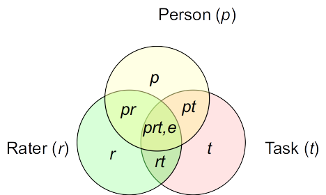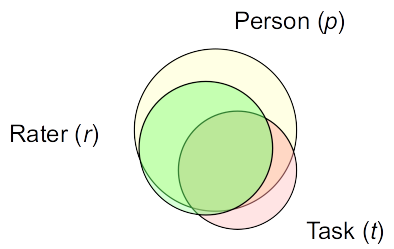### Standard deviationE.g., The ratings are on a 6-point scale. With $\hat \sigma_{pr}$ = `r sqrt(vc_m1$vcov[2])`, this is the margin of error due to rater-by-person interaction, which is not trivial.## Treating Task as Fixed```{r}# If treating task as fixed, the person x task variance will be averaged # and become part of the universe scorevaru <- vc_m1$vcov[3] + vc_m1$vcov[1] /3# The rater x task variance will be averaged and become part of rater variancevarr <- vc_m1$vcov[6] + vc_m1$vcov[4] /3# The residual will be averaged and become part of person x rater variancevare <- vc_m1$vcov[2] + vc_m1$vcov[7] /3# Combinedata.frame(source = vc_m1$grp[c(3, 6, 2)],var =c(varu, varr, vare),percent =c(varu, varr, vare) /sum(varu, varr, vare))```## G and $\phi$ Coefficients```{r}mean_scores <-rowMeans(sample_data[-1])dep_coef <-function(x) { vc_x <-as.data.frame(VarCorr(x))# G coefficient (for relative decision) g_coef <-with( vc_x, vcov[3] / (vcov[3] + vcov[1] /3+ vcov[2] /3+ vcov[7] /3/3) )# phi coefficient (for absolute decision) phi_coef <-with( vc_x, vcov[3] / (vcov[3] + vcov[1] /3+ vcov[2] /3+ vcov[7] /3/3+ vcov[4] /3/3+ vcov[5] /3+ vcov[6] /3) )c(g = g_coef, phi = phi_coef)}dep_coef(m1)```

