Provide some example applications of the generalizability theory (G theory)
Contrast G theory with CTT (Table 10.1)
Explain the differences between crossed and nested facets, and between random and fixed facets, and between G studies and D studies
Estimate variance components and the G and \(\phi\) coefficients for two facets designs
library(here)library(haven) # for reading SPSS datalibrary(tidyverse)library(lme4)
Warning in check_dep_version(): ABI version mismatch:
lme4 was built with Matrix ABI version 2
Current Matrix ABI version is 1
Please re-install lme4 from source or restore original 'Matrix' package
Basic Concepts of G theory
Premise: there are multiple sources of error, and typically observed scores only reflect some specific conditions (e.g., one rater, two trials)
Goal: investigate whether observed scores under one set of conditions can be generalized to broader conditions.
Common Applications
Rating data: Interrater reliability is a special case of G theory.
Behavioral observations: generalizability across different raters, tasks, occasions, intervals of observations, etc.
Imaging data: generalizability of scores across different processing decisions, tasks, etc.
Terminology
Facet: sources of error (e.g., raters, tasks, occasions). Each facet can be fixed or random.
Condition: level of a facet
Object of Measurement: usually people, which is not considered a facet. This is always random.
Universe of Admissible Operations (UAO): a broad set of conditions to which the observed scores generalize
Universerse Score: average score of a person across all possible sets of conditions in the UAO
G Study: obtain accurate information on the magnitude of sources of error
D study: design measurement scenario with the desired level of dependability with the smallest number of conditions
In G theory, by evaluating the degree of error in different sources, we have evidence on whether scores from some admissible conditions are generalizable across conditions. If so, the scores are dependable (or reliable).
One-Facet Design
The example in the previous note with each participant rated by the same set of raters is an example of a one-facet design.
The other facets (rater, task) are embedded in the columns
While it’s possible to run analyses using the wide format, for our analyses we’ll transform the data to a long format as it better suits the analytic framework (variance components model) we’ll use. This also has better handling for missing data.
We’ll use the pivot_longer() function from the tidyr package (which is loaded with library(tidyverse)).
Long Format
Each row represents an observation (repeated measure)
Each facet (rater, task) has its own column
rpa_long <- rpa_dat |>select(id, day, rpa1:rpa3) |>pivot_longer(# select all columns, except the 1st one to be transformedcols = rpa1:rpa3,# The columns have a pattern "rpa(d)", where values# in parentheses are the IDs for the facet. So we first# specify this pattern, with a "." meaning a one-digit# place holder,names_pattern ="rpa(.)",# and then specify that the place holder is for item.names_to =c("item"),values_to ="rpa"# name of score variable)head(rpa_long)
As can be seen, the data are now in a long format.
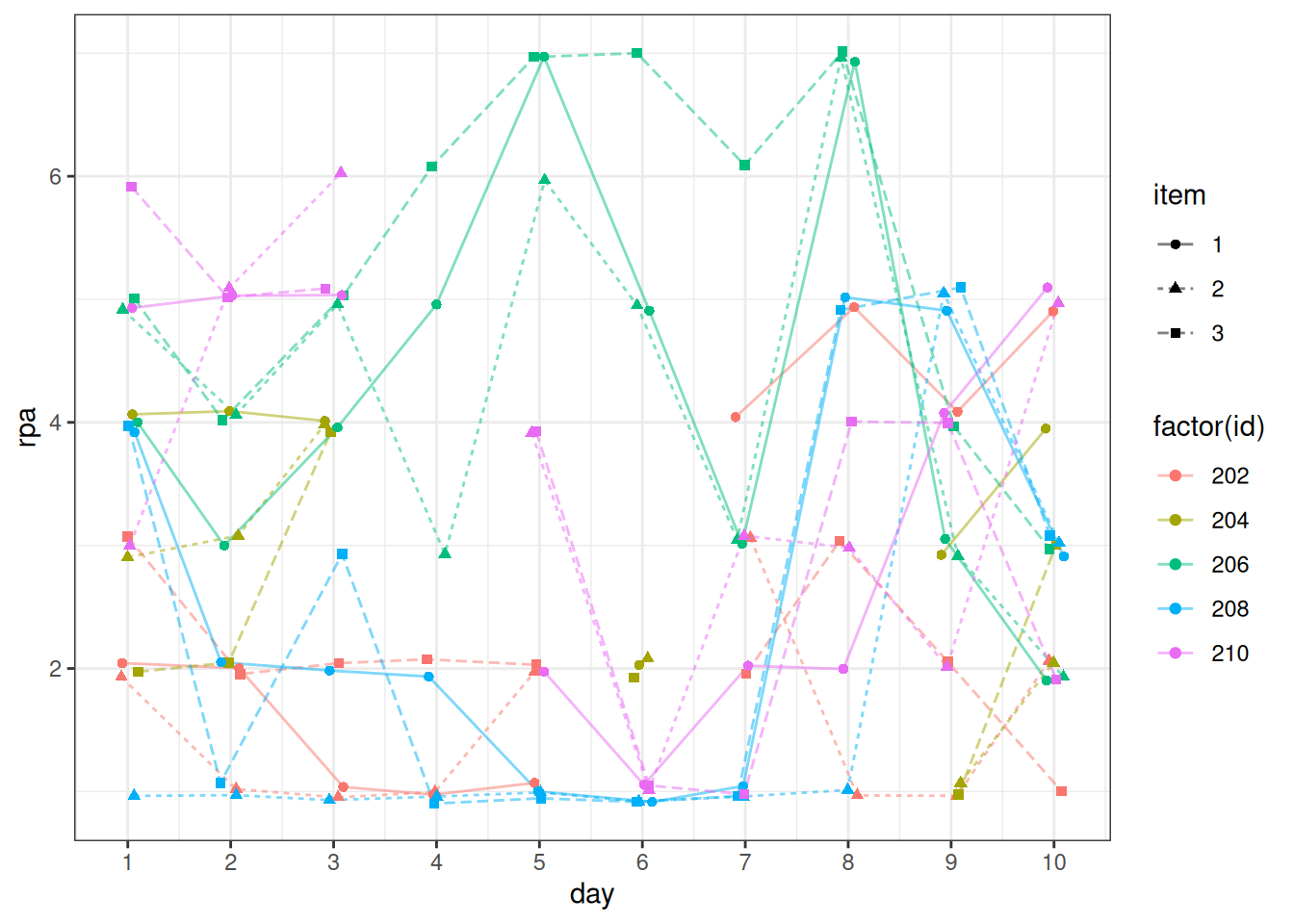
The data here has each participant (p) answering same three items (i) on 10 days (t). However, the participants do not share the same 10 calendar days or days of week, so unless one is interested in day of study effect, one would consider day 2 of Participant A to be different from day 2 of Participant B. Therefore, this is a (t:p) \(\times\)i design, where the two facets are nested.
When facet A is nested in facet B (i.e., a:b), each level of A is associated with only one level of B, but each level of B is associated with multiple levels of A.
Variance Decomposition
With a two-facet design, we have the following variance components:
Person
Facet A
Facet B
Person \(\times\) A
Person \(\times\) B
A \(\times\) B
Person \(\times\) A \(\times\) B*
Error*
*The variances due to Person \(\times\) A \(\times\) B interaction and random error can only be separated when there is more than one observation for each cell (i.e., combination of person, A, and B), which is uncommon.
With a nested design, one cannot estimate the t:i interaction, and the main effect of t and the t:p interaction cannot be separated (See Table 10.6).
m1 <-lmer( rpa ~1+ (1| day:id) + (1| id) + (1| item) + (1| id:item),data = rpa_long)# Variance components (VCs)vc_m1 <-as.data.frame(VarCorr(m1))# Organize in a table, similar to Table 10.4vc_tab <-data.frame(source = vc_m1$grp,var = vc_m1$vcov,percent = vc_m1$vcov /sum(vc_m1$vcov))knitr::kable(vc_tab, digits =2)
Warning in attr(x, "align"): 'xfun::attr()' is deprecated.
Use 'xfun::attr2()' instead.
See help("Deprecated")
Warning in attr(x, "format"): 'xfun::attr()' is deprecated.
Use 'xfun::attr2()' instead.
See help("Deprecated")
source
var
percent
day:id
0.87
0.32
id:item
0.39
0.14
id
0.58
0.21
item
0.07
0.02
Residual
0.84
0.31
Bootstrap Standard Errors and Confidence Intervals
E.g., The ratings are on a 7-point scale. With \(\hat \sigma_{pr}\) = 0.622, this is the margin of error due to person-by-item interaction.
Fixed vs. Random
Generally G theory treats conditions of a facet as random, meaning they are regarded as a random sample from a population collection of samples. However, if such an assumption does not make sense, such as when people are always going to be evaluated on the same tasks, and there is no intention to generalize beyond those tasks, the task facet should be treated as fixed. Then there are two options:
If it makes sense to average the different conditions in a fixed facet (e.g., average score across tasks), follow the code below.
Otherwise, perform a separate G study for each condition of the fixed facet.
If treating item as fixed, the person \(\times\) item variance will be averaged and become part of the universe score
varu <- vc_m1$vcov[3] + vc_m1$vcov[2] /3
The residual will be averaged and become part of person \(\times\) time variance
See Cranford et al. (2006) for similar discussion of generalizability coefficients in longitudinal data.
However, for reliability more comparable to \(\alpha\) and \(\omega\) reliability coefficients, see Lai (2021).
Note on Notation
The caret (^) symbol in \(\hat \sigma^2\) indicate that it is an estimate from the sample.
In D studies, we typically use \(n'\) to represent number of conditions for a facet to be used when designing the study. For example, with the two-facet crossed design with raters and tasks,
---title: "Generalizability Theory"---```{r}#| echo: false# Define a function for formatting numberscomma <-function(x, d =2) format(x, digits = d, big.mark =",")```## Learning Objectives- Provide some example applications of the generalizability theory (G theory)- Contrast G theory with CTT (Table 10.1)- Explain the differences between *crossed* and *nested* facets, and between *random* and *fixed* facets, and between *G studies* and *D studies*- Estimate variance components and the G and $\phi$ coefficients for two facets designs```{r}#| message: falselibrary(here)library(haven) # for reading SPSS datalibrary(tidyverse)library(lme4)```## Basic Concepts of G theoryPremise: there are *multiple* sources of error, and typically observed scores only reflect some specific conditions (e.g., one rater, two trials)Goal: investigate whether observed scores under one set of conditions can be generalized to broader conditions.## Common Applications- **Rating data:** Interrater reliability is a special case of G theory.- **Behavioral observations:** generalizability across different raters, tasks, occasions, intervals of observations, etc.- **Imaging data:** generalizability of scores across different processing decisions, tasks, etc.## Terminology::: {.callout-important appearance="simple"}*Facet*: sources of error (e.g., raters, tasks, occasions). Each facet can be fixed or random.*Condition*: level of a facet*Object of Measurement*: usually people, which is not considered a facet. This is always random.*Universe of Admissible Operations (UAO)*: a broad set of conditions to which the observed scores generalize*Universerse Score*: average score of a person across all possible sets of conditions in the UAO*G Study*: obtain accurate information on the magnitude of sources of error*D study*: design measurement scenario with the desired level of dependability with the smallest number of conditions:::---::: {.callout-tip appearance="simple"}In G theory, by evaluating the degree of error in different sources, we have evidence on whether scores from some admissible conditions are generalizable across conditions. If so, the scores are *dependable* (or reliable).:::## One-Facet DesignThe example in the [previous note](/r-notes/06-irr.qmd) with each participant rated by the same set of raters is an example of a one-facet design.Formula for score of person $i$ by rater $j$:$$\begin{aligned} Y_{ij} & = \mu & \text{(universe score)} \\ & \quad + (\mu_p - \mu) & \text{(person effect)} \\ & \quad + (\mu_r - \mu) & \text{(rater effect)} \\ & \quad + (Y_{ij} - \mu_p - \mu_r + \mu) & \text{(residual)}\end{aligned}$$---This gives the variance decomposition for three components:$$\sigma^2(Y_{pr}) = \sigma^2_p + \sigma^2_r + \sigma^2_{pr, e}$$$\sigma^2_p$ is person variance, or *universe score variance*.Model of analysis: two-way random-effect ANOVA, aka random-effect model, variance component models, or multilevel models with crossed random effects. ## Two-Facet DesignThe first example comes from [a daily diary study](https://onlinelibrary.wiley.com/doi/full/10.1111/jopy.12897) on daily rumination.- <https://osf.io/gnsu2>---*n* = 178, *T* = 10 days- `rpa1`: I often thought of how good I felt today.- `rpa2`: I often thought of how strong I felt today.- `rpa3`: I often thought today that I would achieve everything.```{r}# Import data directly from osf.iorpa_csv <- here::here("data", "rpa_data.csv")if (!file.exists(rpa_csv)) {download.file("https://osf.io/download/gnsu2/",destfile = rpa_csv )}rpa_dat <-read.csv(rpa_csv)rpa_dat |> dplyr::select(id, day, rpa1:rpa3) |> dplyr::glimpse()```## Data TransformationThe data are in a typical *wide format*.::: {.callout-important}## Wide Format- Each row represents a person- The other facets (rater, task) are embedded in the columns:::::: {.content-hidden when-format="revealjs"}While it's possible to run analyses using the wide format, for our analyses we'll transform the data to a long format as it better suits the analytic framework (variance components model) we'll use. This also has better handling for missing data.We'll use the `pivot_longer()` function from the `tidyr` package (which is loaded with `library(tidyverse)`).:::::: {.callout-important}## Long Format- Each row represents an observation (repeated measure)- Each facet (rater, task) has its own column:::---```{r}#| echo: truerpa_long <- rpa_dat |>select(id, day, rpa1:rpa3) |>pivot_longer(# select all columns, except the 1st one to be transformedcols = rpa1:rpa3,# The columns have a pattern "rpa(d)", where values# in parentheses are the IDs for the facet. So we first# specify this pattern, with a "." meaning a one-digit# place holder,names_pattern ="rpa(.)",# and then specify that the place holder is for item.names_to =c("item"),values_to ="rpa"# name of score variable)head(rpa_long)```As can be seen, the data are now in a *long format*.---```{r}rpa_long |>filter(id %in%unique(id)[1:5]) |>arrange(id, item, day) |>ggplot(aes(x = day, y = rpa, color =factor(id), shape = item, linetype = item)) +geom_line(alpha =0.5, position =position_jitter(width =0.1, height =0.1, seed =211)) +geom_point(position =position_jitter(width =0.1, height =0.1, seed =211)) +scale_x_continuous(breaks =1:10) +theme_bw()```# Nested vs. Crossed## Crossed DesignSee [Example 2](/r-notes/07b-gt-part2.qmd#crossed-design) in the other note## Nested DesignThe data here has each participant (*p*) answering same three items (*i*) on 10 days (*t*). However, the participants do not share the same 10 calendar days or days of week, so unless one is interested in day of study effect, one would consider day 2 of Participant A to be different from day 2 of Participant B. Therefore, this is a (*t*:*p*) $\times$ *i* design, where the two facets are nested.::: {.callout-note appearance="simple"}When facet A is nested in facet B (i.e., *a*:*b*), each level of A is associated with only one level of B, but each level of B is associated with multiple levels of A.:::## Variance Decomposition {.smaller}With a two-facet design, we have the following variance components:- Person- Facet A- Facet B- Person $\times$ A- Person $\times$ B- A $\times$ B- Person $\times$ A $\times$ B*- Error*::: aside*The variances due to Person $\times$ A $\times$ B interaction and random error can only be separated when there is more than one observation for each cell (i.e., combination of person, A, and B), which is uncommon. :::---With a nested design, one cannot estimate the *t*:*i* interaction, and the main effect of *t* and the *t*:*p* interaction cannot be separated (See Table 10.6).```{r}m1 <-lmer( rpa ~1+ (1| day:id) + (1| id) + (1| item) + (1| id:item),data = rpa_long)# Variance components (VCs)vc_m1 <-as.data.frame(VarCorr(m1))# Organize in a table, similar to Table 10.4vc_tab <-data.frame(source = vc_m1$grp,var = vc_m1$vcov,percent = vc_m1$vcov /sum(vc_m1$vcov))knitr::kable(vc_tab, digits =2)```## Bootstrap Standard Errors and Confidence IntervalsSee [Part 2 of the notes](/r-notes/07b-gt-part2.qmd#bootstrap-standard-errors-and-confidence-intervals).## Interpreting the Variance Components### Venn diagrams:::: {.columns}::: {.column width="50%"}:::::: {.column width="50%"}:::::::---### Standard deviationE.g., The ratings are on a 7-point scale. With $\hat \sigma_{pr}$ = `r sqrt(vc_m1$vcov[2]) |> round(digits = 3)`, this is the margin of error due to person-by-item interaction.## Fixed vs. Random {.smaller}Generally G theory treats conditions of a facet as random, meaning they are regarded as a random sample from a population collection of samples. However, if such an assumption does not make sense, such as when people are always going to be evaluated on the same tasks, and there is no intention to generalize beyond those tasks, the task facet should be treated as fixed. Then there are two options:a. If it makes sense to average the different conditions in a fixed facet (e.g., average score across tasks), follow the code below.b. Otherwise, perform a separate G study for each condition of the fixed facet. ---If treating item as fixed, the person $\times$ item variance will be averaged and become part of the universe score```{r}varu <- vc_m1$vcov[3] + vc_m1$vcov[2] /3```The residual will be averaged and become part of person $\times$ time variance```{r}vare <- vc_m1$vcov[1] + vc_m1$vcov[5] /3# Combinedata.frame(source = vc_m1$grp[c(3, 1)],var =c(varu, vare),percent =c(varu, vare) /sum(varu, vare))```## Relative vs. Absolute Decisions- Error for relative: anything that involves person, including the residual * $\sigma^2_{pi}$ + $\sigma^2_{pt}$ + $\sigma^2_{pit, e}$- Error for absolute: every term other than person * $\sigma^2_i$ + $\sigma^2_t$ + $\sigma^2_{pi}$ + $\sigma^2_{pt}$ + $\sigma^2_{it}$ + $\sigma^2_{pit, e}$## D StudiesDecision studies: Based on the results of G studies, try to minimize error as much as possible.- Find out how many conditions can be used to optimize generalizability- Similar to using the Spearman-Brown prophecy formula, but consider multiple sources of errors## G and $\phi$ CoefficientsG coefficient: For relative decisions- Only include sources of variation that would change relative standing as error ($\sigma^2_\text{REL}$) * i.e., interaction terms that involve persons$$G = \frac{\hat \sigma^2_p}{\hat \sigma^2_p + \hat \sigma^2_\text{REL}}$$---$\phi$ coefficient: For absolute decisions- Include all sources of variation, except for the one due to persons, as error ($\sigma^2_\text{ABS}$)$$\phi = \frac{\hat \sigma^2_p}{\hat \sigma^2_p + \hat \sigma^2_\text{ABS}}$$These are analogous to (but not the same as) reliability coefficients.---```{r}mean_scores <-tapply(rpa_long$rpa, INDEX = rpa_long$id, FUN = mean, na.rm =TRUE)hist(mean_scores, main ="Estimate of universe score", xlab ="y-bar")``````{r}# G coefficient (for relative decision)g_coef <-with(as.data.frame(VarCorr(m1)), vcov[3] / (vcov[3] + vcov[1] /10+ vcov[2] /3+ vcov[5] / (10*3)))# phi coefficient (for absolute decision)phi_coef <-with(as.data.frame(VarCorr(m1)), vcov[3] / (vcov[3] + vcov[1] /10+ vcov[2] /3+ vcov[4] /3+ vcov[5] / (10*3)))c(g = g_coef, phi = phi_coef)```---See [Cranford et al. (2006)](https://pmc.ncbi.nlm.nih.gov/articles/PMC2414486/pdf/nihms50383.pdf) for similar discussion of generalizability coefficients in longitudinal data.However, for reliability more comparable to $\alpha$ and $\omega$ reliability coefficients, see [Lai (2021)](https://quantscience.rbind.io/postprint/Lai_2020_pm_mcfa_reliability_am.pdf).## Note on NotationThe caret (^) symbol in $\hat \sigma^2$ indicate that it is an estimate from the sample.In D studies, we typically use $n'$ to represent number of conditions for a facet *to be used* when designing the study. For example, with the two-facet crossed design with raters and tasks,$$\hat \sigma^2_\text{REL} = \frac{\sigma^2_{pr}}{n'_r} + \frac{\sigma^2_{pt}}{n'_t} + \frac{\sigma^2_{prt, e}}{n'_r n'_t}$$