library(tidyverse)library(lavaan)library(semPlot, include.only ="semPaths") # for plotting
Warning in check_dep_version(): ABI version mismatch:
lme4 was built with Matrix ABI version 2
Current Matrix ABI version is 1
Please re-install lme4 from source or restore original 'Matrix' package
library(modelsummary, include.only ="msummary")library(semTools, include.only ="compRelSEM") # for composite reliabilitylibrary(semptools) # for adjusting plotslibrary(flextable) # for tableslibrary(psych)
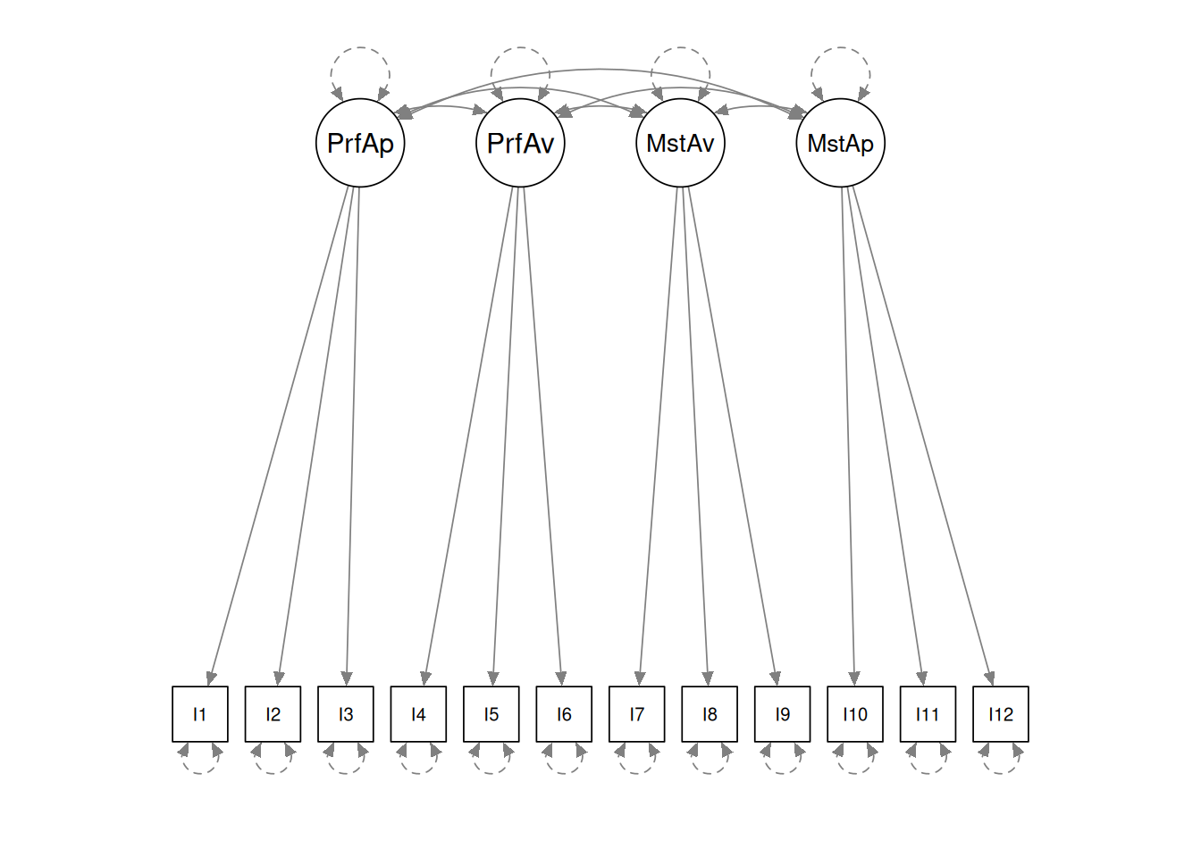
# If using just syntax, need to call `lavaanify()` firstsemPlot::semPaths(lavaanify(cfa_mod))
Model Estimation
Use the lavaan::cfa() function
Use the first item as the reference indicator
# Default of lavaan::cfacfa_fit <-cfa(cfa_mod,sample.cov = covy,# number of observationssample.nobs =1022,# default option to correlate latent factorsauto.cov.lv.x =TRUE,# Model identified by fixing the loading of first indicator to 1std.lv =FALSE)
Standardize latent variable
Technically speaking, this is still not fully identified, because the results will be the same with \(\symbf \Lambda* = -\symbf \Lambda\)
# Default of lavaan::cfacfa_fit2 <-cfa(cfa_mod,sample.cov = covy,# number of observationssample.nobs =1022,# Model identified by standardizing the latent variablesstd.lv =TRUE)
As can be seen below, the two ways of identification give the same implied covariance matrix, but the estimates are different because the latent variables are in different units.
# Implied covariancelavInspect(cfa_fit, what ="cov.ov") -lavInspect(cfa_fit2, what ="cov.ov")
Table 2: Factor correlations of the latent variables.
1
2
3
4
1.PerfAppr
2.PerfAvoi
0.53
3.MastAvoi
0.24
0.50
4.MastAppr
0.30
0.09
0.30
Sample Write-up
We fit a 4-factor model with each item loading on one of the four factors: Performance Approach (Items 1 to 3), Performance Avoidance (Items 4 to 6), Mastery Avoidance (Items 7 to 9), and Mastery Approach (Items 10 to 12). We used the lavaan package (v0.6.19; Rosseel, 2012) with normal distribution-based maximum likelihood estimation. There were no missing data as all participants responded to all items. We evaluate the model using the global \(\chi^2\) test, as well as goodness-of-fit indices including RMSEA (≤ .05 indicating good fit; Browne & Cudeck, 1993), CFI (≥ .95 indicating good fit; Hu & Bentler, 1999), and SRMR (≤ .08 indicating acceptable fit; Hu & Bentler, 1999). We also consider the correlation residuals and the modification indices.
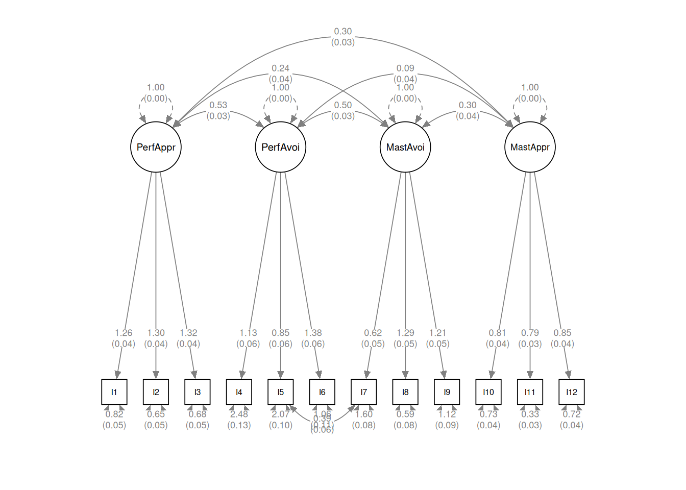
The \(\chi^2\) test indicated that the hypothesized 4-factor model does not perfectly fit the data, \(\chi^2\)(N = 1022, df = 48) = 284, p < .001. However, the fit is reasonable, with RMSEA = .07, 90% CI [.06, .08], CFI = .95, and SRMR = .05. Inspection of the correlation residuals shows relatively large unmodelled correlations between Items 5 and 7 (0.21), and modification indices similarly suggest adding unique covariance between those two items (MI = 40.3961327).
Given that the two items have similar wordings, we refit the model with unique covariance between them. The model fit improves, \(\chi^2\)(N = 1022, df = 47) = 242, p < .001, RMSEA = .06, 90% CI [.06, .07], CFI = .96, and SRMR = .04. Further inspection of correlation residuals and modification indices does not suggest modifications to the model that are theoretically justified.
Figure 1, Table 1, and Table 2 show the parameter estimates of the loadings and uniqueness, based on the final model. When forming composites for the four latent factors, the omega coefficient for the composite reliability is .87 for Performance Approach, .65 for Performance Avoidance, .74 for Mastery Avoidance (Items 7 to 9), and .77 for Mastery Approach.
Example 2: Non-normal Data
Note that methods such MLR and WLSMV require the input of either (a) the raw data or (b) an asymptotic covariance matrix for the sample covariances. We’ll use the bfi data set as an example here.
The parameter estimates with ML (MLM, MLR, etc) and WLS (WLSMV, etc) cannot be directly compared when the parameters involve the observed variables, because these estimation methods treat the variables on different metrics. The factor correlations, on the other hand, can be compared.
Warning in attr(x, "align"): 'xfun::attr()' is deprecated.
Use 'xfun::attr2()' instead.
See help("Deprecated")
MLR
WLSMV
Est.
S.E.
Est.
S.E.
Ag =~ A1
0.520
0.033
0.408
0.019
Ag =~ A2
−0.775
0.027
−0.722
0.013
Ag =~ A3
−0.973
0.029
−0.787
0.012
Ag =~ A4
−0.733
0.032
−0.570
0.017
Ag =~ A5
−0.791
0.027
−0.676
0.014
Co =~ C1
0.668
0.032
0.595
0.016
Co =~ C2
0.801
0.032
0.664
0.014
Co =~ C3
0.715
0.028
0.593
0.015
Co =~ C4
−0.915
0.030
−0.722
0.014
Co =~ C5
−0.965
0.035
−0.644
0.014
Ag ~~ Co
−0.341
0.028
−0.371
0.022
Num.Obs.
2800
2632
AIC
90191.5
BIC
90375.6
# Fit indicessummary( semTools::compareFit(cfa_ac_mlr, cfa_ac_wls, nested =FALSE))
Warning in semTools::compareFit(cfa_ac_mlr, cfa_ac_wls, nested = FALSE):
fitMeasures() returned vectors of different lengths for different models,
probably because certain options are not the same. Check lavInspect(fit,
"options")[c("estimator","test","meanstructure")] for each model, or run
fitMeasures() on each model to investigate.
####################### Model Fit Indices ###########################
           chisq.scaled df.scaled pvalue.scaled rmsea.robust cfi.robust
cfa_ac_mlr     466.460†        34          .000        .073†      .910†
cfa_ac_wls     593.496         34          .000        .087       .905
           tli.robust  srmr
cfa_ac_mlr      .880† .043†
cfa_ac_wls      .875  .051
Weight Matrix (Asymptotic Covariance Matrix of the Sample Covariance Matrix)
[This and the remainder contains more mathematical details.]
Estimators like MLM, MLR, and WLSMV make use of the asymptotic covariance matrix, which is called NACOV or gamma in lavaan. This is an estimated covariance matrix for the sample statistics, and is generally huge in size. For example, if the input matrix is 10 × 10, there are 55 unique variances/covariances, so the asymptotic matrix is 55 × 55.
# Refit with listwise deletion and MLM so that# we don't worry about missing data herecfa_ac_mlm <-cfa( ac_mod,data = bfi,estimator ="MLM")ac_gamma_mlm <-lavInspect(cfa_ac_mlm, what ="gamma")dim(ac_gamma_mlm)
[1] 55 55
Each element of the matrix is a covariance of the covariance. First, note that the covariance is
dat <-lavInspect(cfa_ac_mlm, what ="data")# First, center the datadat_c <-scale(dat, center =TRUE, scale =FALSE)# For example, covariance of (a) cov(A1, A2) and (b) cov(A3, A4)mean(dat_c[, 1] * dat_c[, 2] * dat_c[, 3] * dat_c[, 4]) -cov(dat_c[, 1], dat_c[, 2]) *cov(dat_c[, 3], dat_c[, 4])
[1] -0.7339502
ac_gamma_mlm["A1~~A2", "A3~~A4"]
[1] -0.7342573
The two values almost match, except that in lavaan, the covariance is computed by dividing by \(N\) (instead of \(N - 1\) as in cov). The following computes the asymptotic covariance matrix:
N <-nobs(cfa_ac_mlm)# Sample covariance S (uncorrected)Sy <-cov(dat) * (N -1) / N# Centered data, and transposeac_gamma_hand <-tcrossprod(apply(dat_c, 1, tcrossprod) -as.vector(Sy)) / N# Remove duplicated elementsunique_Sy <-as.vector(lower.tri(Sy, diag =TRUE))# Check the matrices are the sameall.equal(ac_gamma_hand[unique_Sy, unique_Sy],unname(unclass(ac_gamma_mlm)))
[1] TRUE
# MLM using the sample covariance matrix and the asymptotic covariance matrixcfa(ac_mod,sample.cov =cov(dat),sample.nobs = N,estimator ="MLM",NACOV = ac_gamma_hand[unique_Sy, unique_Sy])
lavaan 0.6-19 ended normally after 40 iterations

  Estimator                                         ML
  Optimization method                           NLMINB
  Number of model parameters                        21

  Number of observations                          2632

Model Test User Model:
                                              Standard      Scaled
  Test Statistic                               503.340     424.760
  Degrees of freedom                                34          34
  P-value (Chi-square)                           0.000       0.000
  Scaling correction factor                                  1.185
    Satorra-Bentler correction
Mathematical and Computational Details
Discrepancy function for Normal-Distribution ML
Let \(\boldsymbol{\eta} = [\eta_1, \ldots, \eta_q]^\top\) be the latent factors. Without loss of generality, assume that the items are mean-centered. Assume normality, our factor model becomes
The quadratic form \(\symbf y_i^\top \symbf \Sigma^{-1} \symbf y_i\) can be written as \(\mathop{\mathrm{tr}}(\symbf y_i^\top \symbf \Sigma^{-1} \symbf y_i)\) = \(\mathop{\mathrm{tr}}(\symbf \Sigma^{-1} \symbf y_i \symbf y_i^\top)\), which uses a property of the matrix trace.
Specified model (H0)
The log-likelihood of the data, assuming that each participant is independent, is
Because \(\sum_i^N \symbf y_i \symbf y_i^\top\), the sum of cross-products, is \((N - 1) \symbf S\) where \(\symbf S\) is the sample covariance matrix (you should verify this yourself), we can see \(\symbf S\) is sufficient for inference, and
In a saturated model, it can be shown that \(\hat{\symbf\Sigma} = \tilde{\symbf S} = (N - 1) \symbf S / N\) such that the model-implied covariance matrix is the same as the sample covariance matrix. Thus, \(\mathop{\mathrm{tr}}(\hat{\symbf \Sigma}^{-1} \symbf S)\) = \(N \mathop{\mathrm{tr}}(\symbf I) / (N - 1)\) = \(Np / (N - 1)\), and the saturated loglikelihood is
ny * (logdet_sigma - logdet_tilde_s +sum(diag(solve(sigmahat_mat, tilde_s))) - py)
[1] 284.1989
# Compared to the results in lavaancfa_fit@test$standard$stat
[1] 284.1989
In a large sample, \(T\) follows a \(\chi^2\) distribution with degrees of freedom equals \(p (p + 1) / 2 - m\), where \(m\) is the number of parameters in the model.
Note
Maximum likelihood can be used for categorical items, by using a model that treats the data as discrete instead of continuous. The computation is more intensive as the marginal distribution is no longer normal, and involves integrals that usually do not have close-form solutions.
Weighted Least Squares (WLS)
For continuous variables. The vech() operator converts the lower-diagonal elements of the covariance matrix into a vector.
\[
(\symbf s - \boldsymbol \sigma)^\top \symbf W^{-1} (\symbf s - \boldsymbol \sigma)
\]
for some chosen weight matrix \(\symbf W\), which has dimension of \(p (p + 1) / 2 \times p (p + 1) / 2\).
For example, ULS uses an identity matrix as \(\symbf W\), so the above expression reduces to
\[
(\symbf s - \boldsymbol \sigma)^\top (\symbf s - \boldsymbol \sigma)
\]
Below is an example
uls_fit <-cfa(cfa_mod, sample.cov = covy,# number of observationssample.nobs =1022,estimator ="ULS")# Implied covariance matrixsigmahat_uls <-lavInspect(uls_fit, what ="cov.ov")# ULS discrepancy functionsum((sigmahat_uls - covy)^2) /2
[1] 0.9677648
# Verify that the ML solution gives a larger discrepancy# based on the ULS criterionsum((sigmahat_mat - covy)^2) /2
[1] 1.11625
WLS is more commonly used as a fast alternative to maximum likelihood for categorical items. In such a situation, \(\symbf S\) and \(\symbf \Sigma\) are sample and model-implied polychoric correlation matrices, and the weight matrix is estimated based on the fourth moments (which is related to kurtosis) of the items. Taking the inverse of the full matrix, however, is very computationally intensive and unstable, as the matrix is huge (e.g., 78 \(\times\) 78) in our sample. Therefore, most applications use DWLS, the diagonally weighted version of it, where \(\symbf W\) is chosen as a diagonal matrix with the diagonal elements coming from the full matrix.
---title: "Confirmatory Factor Analysis"---<!-- LaTeX Macro -->::: {.content-hidden when-format="latex"}\DeclareMathOperator{\Tr}{tr}\DeclareMathOperator{\vech}{vech}:::<!-- End LaTeX Macro -->```{r}#| echo: false# Define a function for formatting numberscomma <-function(x, d =2) format(x, digits = d, big.mark =",")# Helper for removing leading zerormlead0 <-function(x, digits =2L) { x[] <-gsub("0\\.", "\\.", sprintf(x, fmt ="%#.2f")) x}``````{r}#| message: falselibrary(tidyverse)library(lavaan)library(semPlot, include.only ="semPaths") # for plottinglibrary(modelsummary, include.only ="msummary")library(semTools, include.only ="compRelSEM") # for composite reliabilitylibrary(semptools) # for adjusting plotslibrary(flextable) # for tableslibrary(psych)``````{r}# Input lower-diagonal elements of correlation matrixcory_lower <-c(.690, .702, .712, .166, .245, .188, .163, .248, .179, .380, .293, .421, .416, .482, .377,-.040, .068, .021, .227, .328, .238, .143, .212, .217, .218, .280, .325, .386, .078, .145, .163, .119, .254, .301, .335, .651, .280, .254, .223, .039, .066, .059, .018, .152, .129, .182, .202, .186, .012, -.008, .051, .052, .202, .177, .558, .112, .154, .128, .029, .021, .084, .160, .221, .205, .483, .580)# Also standard deviationssds <-c(1.55, 1.53, 1.56, 1.94, 1.68, 1.72, # typo in Table 13.31.42, 1.50, 1.61, 1.18, 0.98, 1.20)# Make full covariance matrixcovy <-getCov(cory_lower, diagonal =FALSE, sds = sds,names =paste0("I", 1:12))covy````lavaan`: "la"tent "va"riable "an"alysisOperators:- `F1 =~ y1`: `y1` loads on the latent factor `F`- `F1 ~~ F1`: Variance of `F1`- `y1 ~~ y2`: Covariance between `y1` and `y2````{r}# lavaan syntaxcfa_mod <-" # Loadings PerfAppr =~ I1 + I2 + I3 PerfAvoi =~ I4 + I5 + I6 MastAvoi =~ I7 + I8 + I9 MastAppr =~ I10 + I11 + I12 # Factor covariances (can be omitted) PerfAppr ~~ PerfAvoi + MastAvoi + MastAppr PerfAvoi ~~ MastAvoi + MastAppr MastAvoi ~~ MastAppr"cfa_dag <- dagitty::lavaanToGraph(cfa_mod)# dagitty::vanishingTetrads(cfa_dag)```Path Diagram (Pre-Estimation)```{r}# If using just syntax, need to call `lavaanify()` firstsemPlot::semPaths(lavaanify(cfa_mod))```# Model EstimationUse the `lavaan::cfa()` function1. Use the first item as the reference indicator```{r}# Default of lavaan::cfacfa_fit <-cfa(cfa_mod,sample.cov = covy,# number of observationssample.nobs =1022,# default option to correlate latent factorsauto.cov.lv.x =TRUE,# Model identified by fixing the loading of first indicator to 1std.lv =FALSE)```2. Standardize latent variableTechnically speaking, this is still not fully identified, because the results will be the same with $\symbf \Lambda* = -\symbf \Lambda$```{r}# Default of lavaan::cfacfa_fit2 <-cfa(cfa_mod,sample.cov = covy,# number of observationssample.nobs =1022,# Model identified by standardizing the latent variablesstd.lv =TRUE)```As can be seen below, the two ways of identification give the same implied covariance matrix, but the estimates are different **because the latent variables are in different units.**```{r}# Implied covariancelavInspect(cfa_fit, what ="cov.ov") -lavInspect(cfa_fit2, what ="cov.ov")msummary(list(`reference indicator`= cfa_fit,`standardized latent factor`= cfa_fit2))```# Model Fit```{r}summary(cfa_fit2, fit.measures =TRUE)```# Residuals and Modification Indices```{r}resid(cfa_fit2, type ="cor")modindices(cfa_fit2, sort =TRUE, minimum =10)```Because the correlation residuals and modification indices suggest unmodelled correlations between Items 5 and 7, we can modify our model```{r}cfa_modr <-" # Loadings PerfAppr =~ I1 + I2 + I3 PerfAvoi =~ I4 + I5 + I6 MastAvoi =~ I7 + I8 + I9 MastAppr =~ I10 + I11 + I12 # Factor covariances (can be omitted) PerfAppr ~~ PerfAvoi + MastAvoi + MastAppr PerfAvoi ~~ MastAvoi + MastAppr MastAvoi ~~ MastAppr # Unique covariances I5 ~~ I7"cfa_fitr <-cfa(cfa_modr,sample.cov = covy,sample.nobs =1022,std.lv =TRUE)# Check residuals and modification indices againresid(cfa_fitr, type ="cor")modindices(cfa_fitr, sort =TRUE, minimum =10)```# Composite Reliability```{r}(omegas <-compRelSEM(cfa_fitr))```# Reporting## Path DiagramYou can use the `semPlot::semPaths()` function for path diagrams with estimates. To make the plot a bit nicer, try the [`semptools`](https://sfcheung.github.io/semptools/articles/quick_start_cfa.html) package.```{r}#| label: fig-path-agq#| fig-cap: Path diagram of the 4-factor model. Standard errors are indicated in parentheses.p <-semPaths( cfa_fitr,whatLabels ="est",nCharNodes =0,sizeMan =4,node.width =1,edge.label.cex = .65,# Larger marginmar =c(8, 5, 12, 5),DoNotPlot =TRUE)p2 <-set_cfa_layout( p,indicator_order =paste0("I", 1:12),indicator_factor =rep(c("PerfAppr", "PerfAvoi","MastAvoi", "MastAppr"),each =3),# Make covariances more curvedfcov_curve =1.75,# Move loadings downloading_position = .8) |>mark_se(object = cfa_fitr, sep ="\n")plot(p2)```## Table```{r}#| label: tbl-loadings#| tbl-cap: Factor loadings and uniqueness from the 4-factor CFA model.# Extract estimatesparameterEstimates(cfa_fitr) |># filter only loadings and variances dplyr::filter(grepl("^I.*", rhs)) |># Remove unique covariance dplyr::filter(op =="=~"| lhs == rhs) |># select columns dplyr::select(op, rhs, est, ci.lower, ci.upper) |># make loadings and variances in different columns tidyr::pivot_wider(names_from = op,values_from =3:5) |># add rows tibble::add_row(rhs ="Mastery Approach", .before =10) |> tibble::add_row(rhs ="Mastery Avoidance", .before =7) |> tibble::add_row(rhs ="Perform Avoidance", .before =4) |> tibble::add_row(rhs ="Perform Approach", .before =1) |> flextable::flextable() |># Two digitscolformat_double(digits =2) |># Set headingset_header_labels(values =c("item", "Est", "LL", "UL", "Est", "LL", "UL") ) |>add_header_row(values =c("", "Loading", "Uniqueness"),colwidths =c(1, 3, 3) ) |># merge columnsmerge_h_range(i =c(1, 5, 9, 13), j1 =1, j2 =7) |># alignmentalign(i =1, align ="center", part ="header") |>align(i =c(1, 5, 9, 13), align ="center", part ="body")``````{r}#| label: tbl-lv-cor#| tbl-cap: Factor correlations of the latent variables.# Latent correlationscor_lv <-lavInspect(cfa_fitr, what ="cor.lv")# Remove upper partcor_lv[upper.tri(cor_lv, diag =TRUE)] <-NAcor_lv |>as.data.frame() |>rownames_to_column("var") |># Number first columnmutate(var =paste0(1:4, ".", var)) |> flextable::flextable() |>colformat_double(digits =2) |>set_header_labels(values =c("", "1", "2", "3", "4") )```::: {.callout-tip}## Sample Write-up```{r}#| include: falsefm_fit <-fitmeasures(cfa_fit2)fm_fitr <-fitmeasures(cfa_fitr)```We fit a 4-factor model with each item loading on one of the four factors: Performance Approach (Items 1 to 3), Performance Avoidance (Items 4 to 6), Mastery Avoidance (Items 7 to 9), and Mastery Approach (Items 10 to 12). We used the *lavaan* package (v`r packageVersion("lavaan")`; Rosseel, 2012) with normal distribution-based maximum likelihood estimation. There were no missing data as all participants responded to all items. We evaluate the model using the global $\chi^2$ test, as well as goodness-of-fit indices including RMSEA (≤ .05 indicating good fit; Browne & Cudeck, 1993), CFI (≥ .95 indicating good fit; Hu & Bentler, 1999), and SRMR (≤ .08 indicating acceptable fit; Hu & Bentler, 1999). We also consider the correlation residuals and the modification indices.The $\chi^2$ test indicated that the hypothesized 4-factor model does not perfectly fit the data, $\chi^2$(*N* = `r nobs(cfa_fit2)`, *df* = `r cfa_fit2@test$standard$df`) = `r comma(cfa_fit2@test$standard$stat)`, *p* < .001. However, the fit is reasonable, with RMSEA = `r rmlead0(fm_fit["rmsea"])`, 90% CI [`r rmlead0(fm_fit["rmsea.ci.lower"], 3)`, `r rmlead0(fm_fit["rmsea.ci.upper"], 3)`], CFI = `r rmlead0(fm_fit["cfi"], 3)`, and SRMR = `r rmlead0(fm_fit["srmr"], 3)`. Inspection of the correlation residuals shows relatively large unmodelled correlations between Items 5 and 7 (`r comma(resid(cfa_fit2, type = "cor")$cov[5, 7])`), and modification indices similarly suggest adding unique covariance between those two items (MI = `r modindices(cfa_fit2, sort = TRUE, minimum = 10)[1, "mi"]`).Given that the two items have similar wordings, we refit the model with unique covariance between them. The model fit improves, $\chi^2$(*N* = `r nobs(cfa_fit2)`, *df* = `r cfa_fitr@test$standard$df`) = `r comma(cfa_fitr@test$standard$stat)`, *p* < .001, RMSEA = `r rmlead0(fm_fitr["rmsea"])`, 90% CI [`r rmlead0(fm_fitr["rmsea.ci.lower"], 3)`, `r rmlead0(fm_fitr["rmsea.ci.upper"], 3)`], CFI = `r rmlead0(fm_fitr["cfi"], 3)`, and SRMR = `r rmlead0(fm_fitr["srmr"], 3)`. Further inspection of correlation residuals and modification indices does not suggest modifications to the model that are theoretically justified.@fig-path-agq, @tbl-loadings, and @tbl-lv-cor show the parameter estimates of the loadings and uniqueness, based on the final model. When forming composites for the four latent factors, the omega coefficient for the composite reliability is `r rmlead0(omegas[1])` for Performance Approach, `r rmlead0(omegas[2])` for Performance Avoidance, `r rmlead0(omegas[3])` for Mastery Avoidance (Items 7 to 9), and `r rmlead0(omegas[4])` for Mastery Approach.:::# Example 2: Non-normal DataNote that methods such `MLR` and `WLSMV` require the input of either (a) the raw data or (b) an asymptotic covariance matrix for the sample covariances. We'll use the `bfi` data set as an example here. ::: {.callout-danger}The parameter estimates with ML (MLM, MLR, etc) and WLS (WLSMV, etc) cannot be directly compared when the parameters involve the observed variables, because these estimation methods treat the variables on different metrics. The factor correlations, on the other hand, can be compared. :::```{r}ac_mod <-"Ag =~ A1 + A2 + A3 + A4 + A5Co =~ C1 + C2 + C3 + C4 + C5"# MLRcfa_ac_mlr <-cfa( ac_mod,data = bfi,missing ="fiml",estimator ="MLR",std.lv =TRUE)# WLSMV (missing data with listwise)cfa_ac_wls <-cfa( ac_mod,data = bfi,ordered =TRUE,estimator ="WLSMV", # default when `ordered = TRUE`std.lv =TRUE)# Comparemsummary(list(MLR = cfa_ac_mlr, WLSMV = cfa_ac_wls),shape = term ~ model + statistic)# Fit indicessummary( semTools::compareFit(cfa_ac_mlr, cfa_ac_wls, nested =FALSE))```## Weight Matrix (Asymptotic Covariance Matrix of the Sample Covariance Matrix)[This and the remainder contains more mathematical details.]Estimators like MLM, MLR, and WLSMV make use of the asymptotic covariance matrix, which is called `NACOV` or `gamma` in `lavaan`. This is an estimated covariance matrix for the sample statistics, and is generally huge in size. For example, if the input matrix is 10 × 10, there are 55 unique variances/covariances, so the asymptotic matrix is 55 × 55.```{r}# Refit with listwise deletion and MLM so that# we don't worry about missing data herecfa_ac_mlm <-cfa( ac_mod,data = bfi,estimator ="MLM")ac_gamma_mlm <-lavInspect(cfa_ac_mlm, what ="gamma")dim(ac_gamma_mlm)```Each element of the matrix is a **covariance of the covariance**. First, note that the covariance is$$\sigma_{XY} = E\{[X - E(Y)] \times [Y - E(Y)]\}$$The covariance of the covariance is$$\sigma_{ABCD} = E\{[A - E(A)] \times [B - E(B)] \times [C - E(C)] \times [D - E(D)]\} - \sigma_{AB} \sigma_{CD}$$```{r}dat <-lavInspect(cfa_ac_mlm, what ="data")# First, center the datadat_c <-scale(dat, center =TRUE, scale =FALSE)# For example, covariance of (a) cov(A1, A2) and (b) cov(A3, A4)mean(dat_c[, 1] * dat_c[, 2] * dat_c[, 3] * dat_c[, 4]) -cov(dat_c[, 1], dat_c[, 2]) *cov(dat_c[, 3], dat_c[, 4])ac_gamma_mlm["A1~~A2", "A3~~A4"]```The two values almost match, except that in `lavaan`, the covariance is computed by dividing by $N$ (instead of $N - 1$ as in `cov`). The following computes the asymptotic covariance matrix:```{r}N <-nobs(cfa_ac_mlm)# Sample covariance S (uncorrected)Sy <-cov(dat) * (N -1) / N# Centered data, and transposeac_gamma_hand <-tcrossprod(apply(dat_c, 1, tcrossprod) -as.vector(Sy)) / N# Remove duplicated elementsunique_Sy <-as.vector(lower.tri(Sy, diag =TRUE))# Check the matrices are the sameall.equal(ac_gamma_hand[unique_Sy, unique_Sy],unname(unclass(ac_gamma_mlm)))``````{r}# MLM using the sample covariance matrix and the asymptotic covariance matrixcfa(ac_mod,sample.cov =cov(dat),sample.nobs = N,estimator ="MLM",NACOV = ac_gamma_hand[unique_Sy, unique_Sy])```# Mathematical and Computational Details## Discrepancy function for Normal-Distribution MLLet $\boldsymbol{\eta} = [\eta_1, \ldots, \eta_q]^\top$ be the latent factors. Without loss of generality, assume that the items are mean-centered. Assume normality, our factor model becomes$$\begin{aligned} \symbf y | \boldsymbol \eta_q & \sim N_p(\symbf{\Lambda} \boldsymbol \eta_q, \symbf \Theta) \\ \boldsymbol \eta_q & \sim N_p(\symbf 0, \symbf \Theta)\end{aligned},$$which implies that the marginal distribution of $\symbf y$ is also normal:$$\symbf y \sim N_p(\symbf 0, \symbf\Sigma)$$The log-density of $\symbf y_i$ for person $i$, which is multivariate normal of dimension $p$, is$$ \log f(\symbf y_i; \symbf\Sigma) = -\frac{1}{2} \log(2 \pi) - \frac{1}{2} \log |\symbf \Sigma| - \frac{1}{2} \symbf y_i^\top \symbf \Sigma^{-1} \symbf y_i$$The quadratic form $\symbf y_i^\top \symbf \Sigma^{-1} \symbf y_i$ can be written as $\Tr(\symbf y_i^\top \symbf \Sigma^{-1} \symbf y_i)$ = $\Tr(\symbf \Sigma^{-1} \symbf y_i \symbf y_i^\top)$, which uses a property of the matrix trace.### Specified model (H0)The log-likelihood of the data, assuming that each participant is independent, is$$\begin{aligned} \ell(\symbf\Sigma; \symbf y_i, \ldots, \symbf y_N) & = - \frac{Np}{2} \log(2\pi) - \frac{N}{2} \log |\symbf \Sigma| - \frac{1}{2} \sum_i^N \Tr \left(\symbf \Sigma^{-1} \symbf y_i \symbf y_i^\top\right) \\ & = - \frac{Np}{2} \log(2\pi) - \frac{N}{2} \log |\symbf \Sigma| - \frac{1}{2} \Tr\left(\symbf \Sigma^{-1} \sum_i^N \symbf y_i \symbf y_i^\top\right)\end{aligned}$$Because $\sum_i^N \symbf y_i \symbf y_i^\top$, the sum of cross-products, is $(N - 1) \symbf S$ where $\symbf S$ is the sample covariance matrix (you should verify this yourself), we can see $\symbf S$ is sufficient for inference, and$$\ell(\symbf\Sigma; \symbf S) = - \frac{Np}{2} \log(2\pi) - \frac{N}{2} \log |\symbf \Sigma| - \frac{N - 1}{2} \Tr \left(\symbf \Sigma^{-1} \symbf S\right)$$You can verify this in *lavaan*```{r}# Implied covariancesigmahat_mat <-lavInspect(cfa_fit, what ="cov.ov")ny <-1022py <-12# number of itemslogdet_sigma <-as.vector(determinant(sigmahat_mat, log =TRUE)$modulus)ll <--ny * py /2*log(2* pi) - ny /2* logdet_sigma - (ny -1) /2*sum(diag(solve(sigmahat_mat, covy)))print(ll)# Compare to lavaanlogLik(cfa_fit)```::: {.callout-note}## Code ExampleHere is a code example for finding MLE of the above model in R:```{r}# 1. Define a function that converts a parameter vector# to the implied covariancesimplied_cov <-function(pars) {# Initialize Lambda (first indicator fixed to 1) lambda_mat <-matrix(0, nrow =12, ncol =4) lambda_mat[1, 1] <-1 lambda_mat[4, 2] <-1 lambda_mat[7, 3] <-1 lambda_mat[10, 4] <-1# Fill the first eight values of pars to the matrix lambda_mat[2:3, 1] <- pars[1:2] lambda_mat[5:6, 2] <- pars[3:4] lambda_mat[8:9, 3] <- pars[5:6] lambda_mat[11:12, 4] <- pars[7:8]# Fill the next 10 values to the Psi matrix psi_mat <-getCov(pars[9:18])# Fill the Theta matrix theta_mat <-diag(pars[19:30])# Implied covariances lambda_mat %*%tcrossprod(psi_mat, lambda_mat) + theta_mat}# 2. Set initial valuespars0 <-c(# loadingsrep(1, 8),# psi1, .3, 1, .3, .3, 1, .3, .3, .3, 1,# thetarep(1, 12))# 3. Likelihood functionfitfunction_ml <-function(pars, covy, ny =1022) { py <-nrow(covy) sigmahat_mat <-implied_cov(pars) logdet_sigma <-as.vector(determinant(sigmahat_mat, log =TRUE)$modulus)-ny * py /2*log(2* pi) - ny /2* logdet_sigma - (ny -1) /2*sum(diag(solve(sigmahat_mat, covy)))}# fitfunction_ml(pars0, covy)# 4. Optimizationopt <-optim(pars0,fn = fitfunction_ml,covy = covy,method ="L-BFGS-B",# Minimize -2 x llcontrol =list(fnscale =-2))# 5. Resultsopt$par[1:8] # Lambda# Compare to lavaanlavInspect(cfa_fit, what ="est")$lambdagetCov(opt$par[9:18],names =paste0("F", 1:4)) # Psi# Compare to lavaanlavInspect(cfa_fit, what ="est")$psidiag(opt$par[19:30]) # ThetalavInspect(cfa_fit, what ="est")$theta# 6. Maximized log-likelihoodopt$value```:::### Saturated model (H1)In a saturated model, it can be shown that $\hat{\symbf\Sigma} = \tilde{\symbf S} = (N - 1) \symbf S / N$ such that the model-implied covariance matrix is the same as the sample covariance matrix. Thus, $\Tr (\hat{\symbf \Sigma}^{-1} \symbf S)$ = $N \Tr (\symbf I) / (N - 1)$ = $Np / (N - 1)$, and the saturated loglikelihood is$$\ell_1 = \ell(\symbf \Sigma = \symbf S; \symbf S) = - \frac{Np}{2} (\log(2\pi) + 1) - \frac{N}{2} \log |\tilde{\symbf S}| - \frac{Np}{2}$$```{r}tilde_s <- (ny -1) / ny * covylogdet_tilde_s <-as.vector(determinant(tilde_s, log =TRUE)$modulus)ll1 <--ny * py /2*log(2* pi) - ny /2* logdet_tilde_s - ny * py /2print(ll1)```### Likelihood-ratio test statistic ($\chi^2$)$$\begin{aligned} T = -2 [\ell(\hat{\symbf\Sigma}; \symbf S) - \ell_1] & = N \left[\log |\hat{\symbf \Sigma}| - \log |\tilde{\symbf S}| + \Tr \left(\hat{\symbf \Sigma}^{-1}\tilde{\symbf S}\right) - p\right]\end{aligned}$$```{r}ny * (logdet_sigma - logdet_tilde_s +sum(diag(solve(sigmahat_mat, tilde_s))) - py)# Compared to the results in lavaancfa_fit@test$standard$stat```In a large sample, $T$ follows a $\chi^2$ distribution with degrees of freedom equals $p (p + 1) / 2 - m$, where $m$ is the number of parameters in the model.::: {.callout-note}Maximum likelihood can be used for categorical items, by using a model that treats the data as discrete instead of continuous. The computation is more intensive as the marginal distribution is no longer normal, and involves integrals that usually do not have close-form solutions.:::## Weighted Least Squares (WLS)For continuous variables. The vech() operator converts the lower-diagonal elements of the covariance matrix into a vector. $$\begin{aligned} \symbf \sigma & = \vech(\symbf \Sigma) \\ \symbf s & = \vech(\symbf S)\end{aligned}$$For our example, $\vech(\Sigma)$ will have $p (p + 1) / 2$ elements.```{r}lavaan::lav_matrix_vech(covy)# Same ascovy[lower.tri(covy, diag =TRUE)]```WLS finds a solution that minimizes$$(\symbf s - \boldsymbol \sigma)^\top \symbf W^{-1} (\symbf s - \boldsymbol \sigma)$$for some chosen weight matrix $\symbf W$, which has dimension of $p (p + 1) / 2 \times p (p + 1) / 2$.For example, ULS uses an identity matrix as $\symbf W$, so the above expression reduces to$$(\symbf s - \boldsymbol \sigma)^\top (\symbf s - \boldsymbol \sigma)$$Below is an example```{r}uls_fit <-cfa(cfa_mod, sample.cov = covy,# number of observationssample.nobs =1022,estimator ="ULS")# Implied covariance matrixsigmahat_uls <-lavInspect(uls_fit, what ="cov.ov")# ULS discrepancy functionsum((sigmahat_uls - covy)^2) /2# Verify that the ML solution gives a larger discrepancy# based on the ULS criterionsum((sigmahat_mat - covy)^2) /2```WLS is more commonly used as a fast alternative to maximum likelihood for categorical items. In such a situation, $\symbf S$ and $\symbf \Sigma$ are sample and model-implied *polychoric correlation* matrices, and the weight matrix is estimated based on the fourth moments (which is related to kurtosis) of the items. Taking the inverse of the full matrix, however, is very computationally intensive and unstable, as the matrix is huge (e.g., 78 $\times$ 78) in our sample. Therefore, most applications use DWLS, the diagonally weighted version of it, where $\symbf W$ is chosen as a diagonal matrix with the diagonal elements coming from the full matrix. Here is a blog post I wrote about WLS: <https://quantscience.rbind.io/2020/06/12/weighted-least-squares/>