library(tidyverse)
library(psych)
library(dagitty)
library(plotly)
library(lavaan)
library(EFAtools)
library(flextable)Exploratory Factor Analysis
Path Diagram
Personally, it may be easier to use powerpoint or other tools with a graphical interface. But if you want to do it with code, here is an example with Graphviz.
Graphviz
digraph FactorModel {
    node [shape=circle,fontsize=12];
    F1; F2;

    node [shape=rectangle];
    x1; x2; x3; x4; x5; x6;

    edge [fontsize=10];
    F2 -> F1 [label="r" constraint=false dir="both"];
    F1 -> x1 [label="a"];
    F1 -> x2 [label="b"];
    F1 -> x3 [label="c"];
    F1 -> x4 [label="d"]
    F2 -> x4 [label="e"];
    F2 -> x5 [label="f"];
    F2 -> x6 [label="g"];

    node [shape=none,fontsize=10];
    u1 -> x1;
    u2 -> x2;
    u3 -> x3;
    u4 -> x4;
    u5 -> x5;
    u6 -> x6;

    {rank=same; x1 x2 x3 x4 x5 x6}
    {rank=min; F1 F2}
    {rank=max; u1 u2 u3 u4 u5 u6}
}Path diagram of a two-factor model.
DAG
A factor model can also be represented as a directed acyclic graph (DAG). The dagitty package can show the vanishing tetrad assumptions:
dag1 <- dagitty("dag{ F1 -> {1 2 3 4}; F2 -> {4 5 6}; F1 <-> F2 }")
latents(dag1) <- c("F1", "F2")
coordinates(dag1) <- list(
    x = c(F1 = 0, F2 = 2, `1` = -1.5, `2` = -0.5, `3` = 0.5, `4` = 1.5,
          `5` = 2.5, `6` = 3.5),
    y = c(F1 = 0, F2 = 0, `1` = 1, `2` = 1, `3` = 1, `4` = 1,
          `5` = 1, `6` = 1)
)
plot(dag1)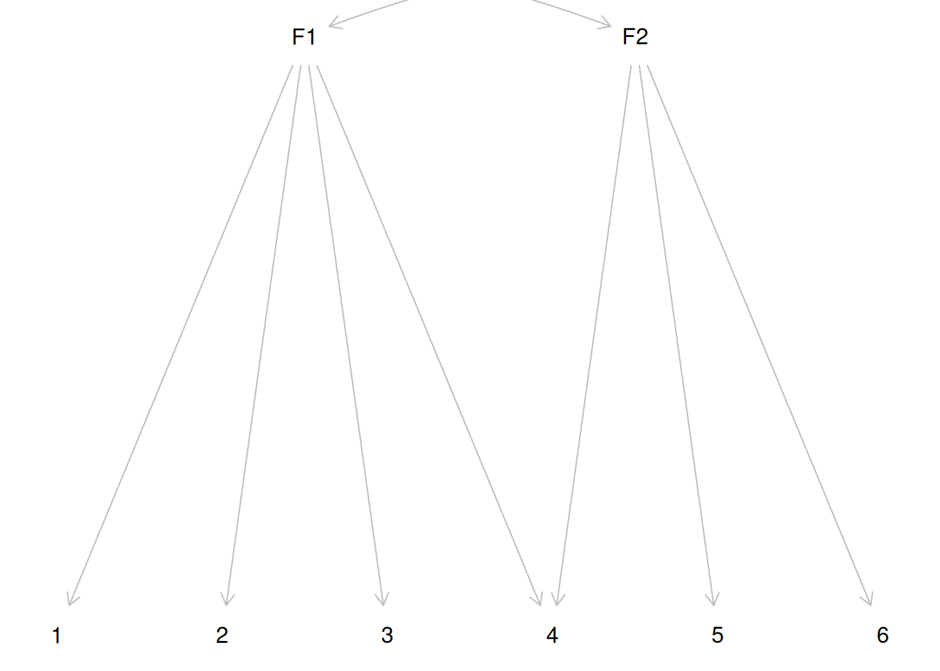
vanishingTetrads(dag1) [,1] [,2] [,3] [,4]
[1,] "1" "3" "4" "2"
[2,] "1" "2" "4" "3"
[3,] "1" "2" "3" "4"
[4,] "1" "3" "5" "2"
[5,] "1" "2" "5" "3"
[6,] "1" "2" "3" "5"
[7,] "1" "3" "6" "2"
[8,] "1" "2" "6" "3"
[9,] "1" "2" "3" "6"
[10,] "1" "4" "5" "2"
[11,] "1" "4" "6" "2"
[12,] "1" "5" "6" "2"
[13,] "1" "4" "5" "3"
[14,] "1" "4" "6" "3"
[15,] "1" "5" "6" "3"
[16,] "1" "5" "6" "4"
[17,] "2" "4" "5" "3"
[18,] "2" "4" "6" "3"
[19,] "2" "5" "6" "3"
[20,] "2" "5" "6" "4"
[21,] "3" "5" "6" "4" Correlation Matrix
# Covariance
cov_oa <- cov(
    select(bfi, O1:O5, A1:A5),
    # Listwise deletion
    use = "complete"
)
# Correlation
corr_oa <- cor(
    select(bfi, O1:O5, A1:A5),
    # Listwise deletion
    use = "complete"
)
round(corr_oa, digits = 2)
O1 O2 O3 O4 O5 A1 A2 A3 A4 A5
O1 1.00 -0.22 0.39 0.19 -0.24 0.01 0.13 0.15 0.06 0.16
O2 -0.22 1.00 -0.28 -0.08 0.33 0.07 0.01 0.00 0.04 -0.01
O3 0.39 -0.28 1.00 0.19 -0.32 -0.06 0.16 0.23 0.07 0.24
O4 0.19 -0.08 0.19 1.00 -0.18 -0.08 0.08 0.04 -0.04 0.02
O5 -0.24 0.33 -0.32 -0.18 1.00 0.11 -0.09 -0.06 0.02 -0.06
A1 0.01 0.07 -0.06 -0.08 0.11 1.00 -0.34 -0.27 -0.15 -0.19
A2 0.13 0.01 0.16 0.08 -0.09 -0.34 1.00 0.49 0.33 0.39
A3 0.15 0.00 0.23 0.04 -0.06 -0.27 0.49 1.00 0.37 0.51
A4 0.06 0.04 0.07 -0.04 0.02 -0.15 0.33 0.37 1.00 0.31
A5 0.16 -0.01 0.24 0.02 -0.06 -0.19 0.39 0.51 0.31 1.00Polychoric Correlation
The items are technically ordinal, but with six points it is usually less a problem to just use Pearson correlation. We can use the lavaan package to get the polychoric correlation.
pcorr_oa <- lavaan::lavCor(select(bfi, O1:O5, A1:A5), ordered = TRUE)
pcorr_oa
O1 O2 O3 O4 O5 A1 A2 A3 A4 A5
O1 1.000
O2 -0.273 1.000
O3 0.450 -0.337 1.000
O4 0.258 -0.106 0.255 1.000
O5 -0.304 0.373 -0.381 -0.250 1.000
A1 -0.010 0.079 -0.086 -0.100 0.134 1.000
A2 0.163 -0.002 0.189 0.109 -0.114 -0.411 1.000
A3 0.187 -0.029 0.270 0.065 -0.089 -0.327 0.565 1.000
A4 0.071 0.035 0.082 -0.049 0.026 -0.182 0.390 0.422 1.000
A5 0.195 -0.018 0.275 0.028 -0.074 -0.234 0.453 0.576 0.358 1.000Heat Map
corr_oa |>
    as_tibble(rownames = "Var1") |>
    pivot_longer(cols = -Var1, names_to = "Var2") |>
    mutate(across(1:2, .fns = as.ordered)) |>
    filter(Var2 > Var1) |>
    ggplot(aes(x = Var2, y = Var1, fill = value)) +
    geom_tile(color = "white") +
    geom_text(aes(Var2, Var1, label = rmlead0(value)), color = "black", size = 4) +
    scale_fill_gradient2(low = "blue", high = "red", limit = c(-1, 1), name = "Pearson\nCorrelation") +
    theme(axis.title.x = element_blank(),
          axis.title.y = element_blank(),
          panel.background = element_blank()) +
    coord_fixed()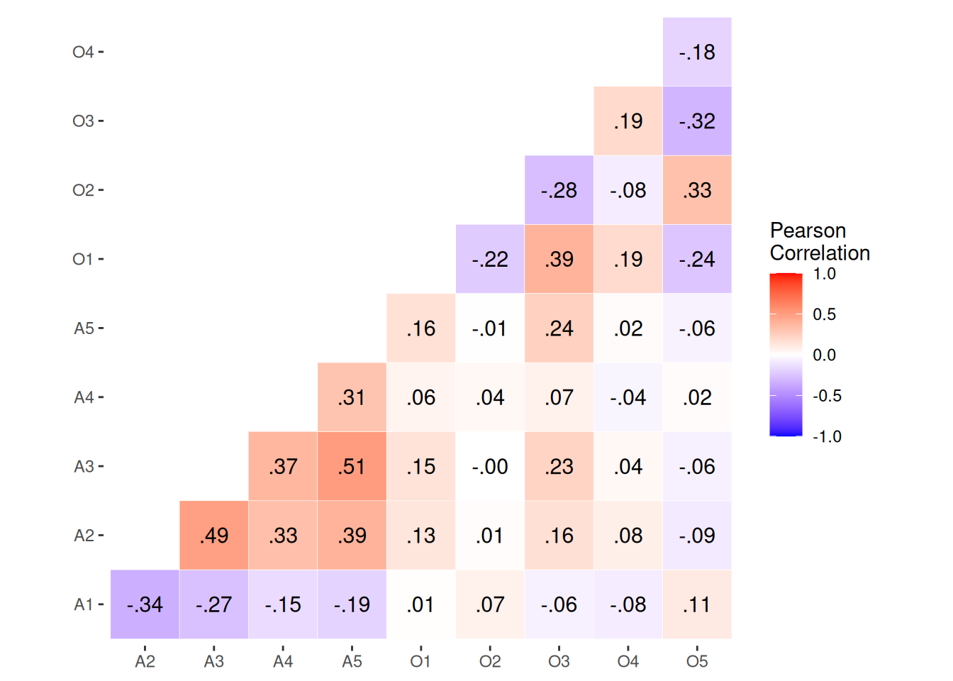
Factor Extraction
Eigen-Decomposition
A good video to explain this: https://www.youtube.com/watch?v=86ODrk1nB-g
# Simulate 3-D Data
lambda_mat <- matrix(c(.8, .7, .5, .1, .5, .4), nrow = 3)
sigma_mat <- tcrossprod(lambda_mat)
diag(sigma_mat) <- 1
y <- MASS::mvrnorm(500, mu = rep(0, 3), Sigma = sigma_mat, empirical = TRUE)
# library(scatterplot3d)
# scatterplot3d(y)
dfy <- as.data.frame(y)
names(dfy) <- c("y1", "y2", "y3")
plot_ly(dfy, x = ~ y1, y = ~ y2, z = ~ y3)No trace type specified:
Based on info supplied, a 'scatter3d' trace seems appropriate.
Read more about this trace type -> https://plotly.com/r/reference/#scatter3dNo scatter3d mode specifed:
Setting the mode to markers
Read more about this attribute -> https://plotly.com/r/reference/#scatter-modeEstimating Communalities
Squared multiple correlations (\(R^2\))
Use squared multiple \(R^2\) (not efficient)
# E.g., Regress A1 on all other variables
summary(lm(A1 ~ ., data = select(bfi, O1:O5, A1:A5)))
Call:
lm(formula = A1 ~ ., data = select(bfi, O1:O5, A1:A5))

Residuals:
    Min      1Q  Median      3Q     Max
-3.5113 -0.9180 -0.3207  0.7330  4.5763

Coefficients:
            Estimate Std. Error t value Pr(>|t|)
(Intercept)  3.95198    0.20993  18.825  < 2e-16 ***
O1           0.12114    0.02488   4.869 1.19e-06 ***
O2           0.07446    0.01761   4.228 2.44e-05 ***
O3           0.04967    0.02429   2.045  0.04098 *
O4          -0.06568    0.02182  -3.010  0.00263 **
O5           0.08494    0.02114   4.018 6.03e-05 ***
A2          -0.32318    0.02565 -12.599  < 2e-16 ***
A3          -0.13979    0.02469  -5.662 1.66e-08 ***
A4          -0.02005    0.01885  -1.063  0.28765
A5          -0.03240    0.02404  -1.348  0.17780
---
Signif. codes:  0 '***' 0.001 '**' 0.01 '*' 0.05 '.' 0.1 ' ' 1

Residual standard error: 1.295 on 2637 degrees of freedom
  (153 observations deleted due to missingness)
Multiple R-squared:  0.1541,    Adjusted R-squared:  0.1512
F-statistic: 53.37 on 9 and 2637 DF,  p-value: < 2.2e-16
# E.g., Regress O1 on all other variables
summary(lm(O1 ~ ., data = select(bfi, O1:O5, A1:A5)))
Call:
lm(formula = O1 ~ ., data = select(bfi, O1:O5, A1:A5))

Residuals:
    Min      1Q  Median      3Q     Max
-4.5570 -0.5727  0.1064  0.7152  2.6925

Coefficients:
             Estimate Std. Error t value Pr(>|t|)
(Intercept)  2.730613   0.165923  16.457  < 2e-16 ***
O2          -0.080779   0.013678  -5.906 3.96e-09 ***
O3           0.264794   0.018230  14.525  < 2e-16 ***
O4           0.098933   0.016922   5.846 5.64e-09 ***
O5          -0.082739   0.016445  -5.031 5.20e-07 ***
A1           0.073559   0.015107   4.869 1.19e-06 ***
A2           0.052696   0.020556   2.564  0.01042 *
A3           0.032197   0.019345   1.664  0.09616 .
A4           0.008584   0.014692   0.584  0.55911
A5           0.049964   0.018712   2.670  0.00763 **
---
Signif. codes:  0 '***' 0.001 '**' 0.01 '*' 0.05 '.' 0.1 ' ' 1

Residual standard error: 1.009 on 2637 degrees of freedom
  (153 observations deleted due to missingness)
Multiple R-squared:  0.2031,    Adjusted R-squared:  0.2004
F-statistic: 74.67 on 9 and 2637 DF,  p-value: < 2.2e-16
A computational short cut is to use the inverse of the correlation matrix
1 - 1 / diag(solve(corr_oa)) O1 O2 O3 O4 O5 A1 A2 A3
0.2030977 0.1625871 0.2766737 0.0766234 0.1910893 0.1540951 0.3401059 0.4002928
A4 A5
0.1885574 0.3138769 Iterative method
Here is sample code for principal axis factoring (using eigen)
rcorr_oa <- corr_oa # initialize reduced correlation
diag(rcorr_oa) <- 1 - 1 / diag(solve(corr_oa))  # replace communality
q <- 2  # number of factors
eps <- .0001  # convergence criterion
while (TRUE) {
    eigen_r <- eigen(rcorr_oa, symmetric = TRUE)
    lambdat <- t(eigen_r$vectors[, seq_len(q)]) * sqrt(eigen_r$values[seq_len(q)])
    # communality = sum of squared loadings
    new_h <- colSums(lambdat^2)
    if (max(abs(new_h - diag(rcorr_oa))) > eps) {
        diag(rcorr_oa) <- new_h
    } else {
        break  # stop when convergence is met
    }
}
# Estimates with the iterative method
diag(rcorr_oa)
O1 O2 O3 O4 O5 A1 A2
0.28265008 0.23396855 0.43541770 0.08877585 0.29766819 0.13249392 0.45364581
A3 A4 A5
0.58815163 0.25098540 0.39616917 The final estimates are different from the initial ones.
Loading Matrix
# From our for loop for PAF
t(lambdat)
[,1] [,2]
[1,] 0.3548181 -0.3959189
[2,] -0.1755868 0.4506955
[3,] 0.4741739 -0.4589373
[4,] 0.1651205 -0.2480128
[5,] -0.2778184 0.4695370
[6,] -0.3486927 -0.1044201
[7,] 0.6303503 0.2372005
[8,] 0.7164531 0.2737558
[9,] 0.4173173 0.2771697
[10,] 0.6018286 0.1842694# Compared to `psych::fa()`
fa_unrotated <- psych::fa(
select(bfi, O1:O5, A1:A5),
nfactors = 2,
rotate = "none",
fm = "pa")
fa_unrotated$loadings
Loadings:
   PA1    PA2
O1  0.356 -0.392
O2 -0.166  0.442
O3  0.472 -0.453
O4  0.163 -0.244
O5 -0.270  0.476
A1 -0.345
A2  0.631  0.231
A3  0.705  0.271
A4  0.415  0.270
A5  0.601  0.187

                 PA1   PA2
SS loadings    2.025 1.084
Proportion Var 0.202 0.108
Cumulative Var 0.202 0.311
The values are not exactly the same as there are differences in implementation algorithms, but they are pretty close.
Number of Factors
Parallel Analysis
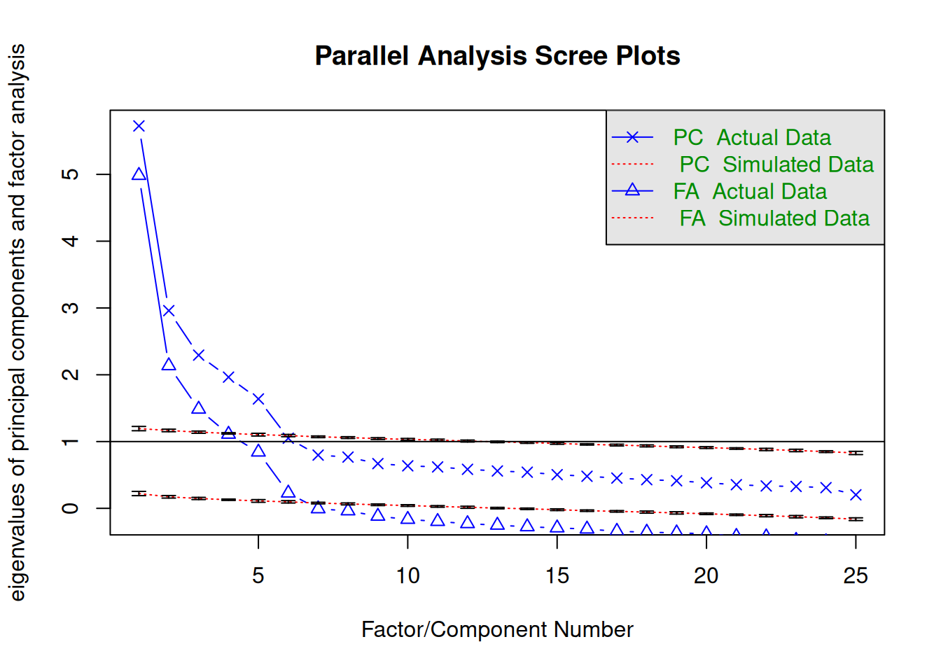
fa.parallel(
    select(bfi, O1:O5, A1:A5),
    fm = "pa",
    error.bars = TRUE
)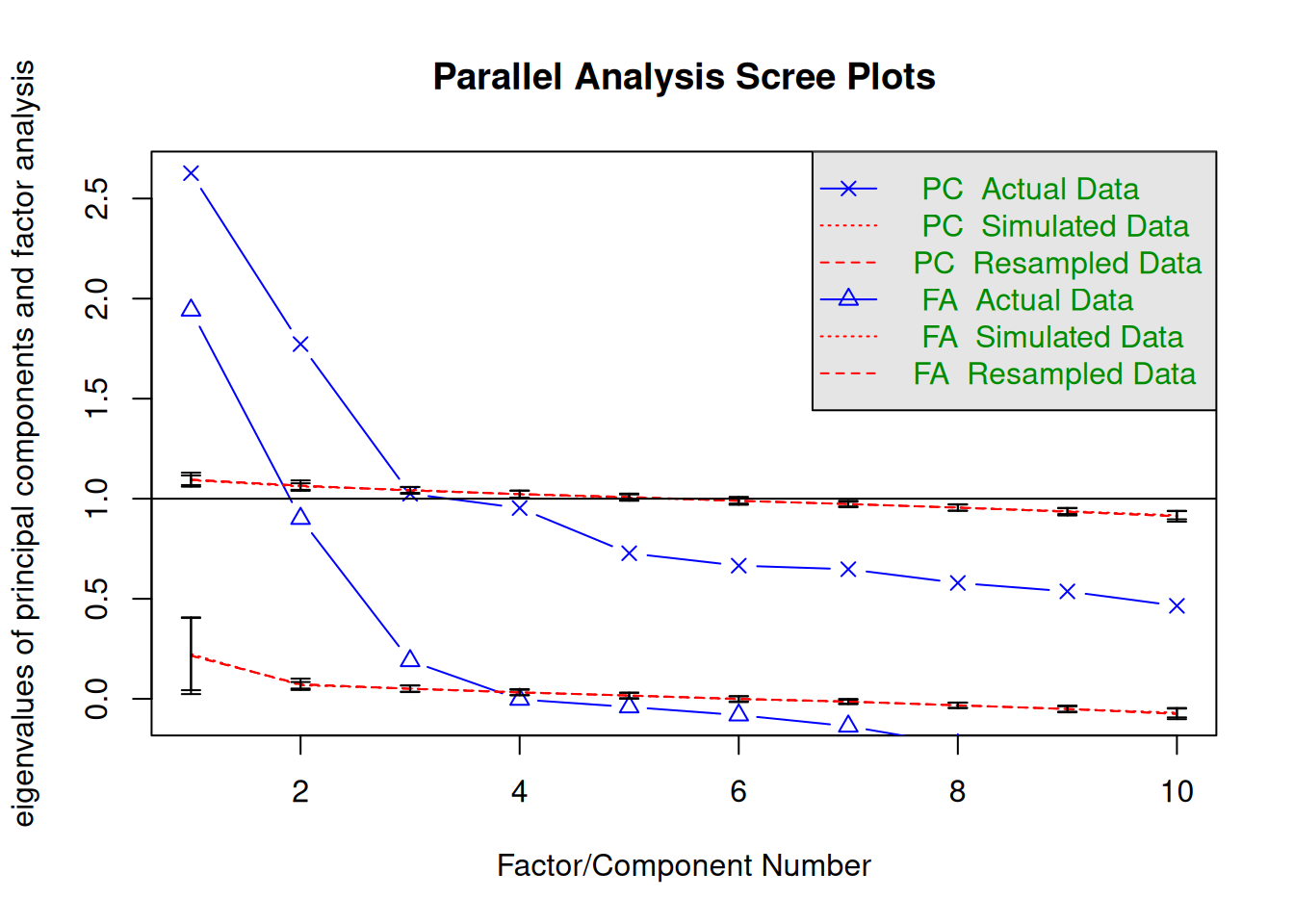
Parallel analysis suggests that the number of factors = 3 and the number of components = 2 It suggests 3 factors (with reduced correlation) and 2 components (with full correlation). In my experience, the number of components is usually more in line with theoretical expectations, but choosing either one would seem reasonable, and this should depend on theoretical considerations and interpretability of the solutions.
With polychoric correlation matrix
We need to first find the number of observations:
n_pcorr <-
    select(bfi, O1:O5, A1:A5) |>
    drop_na() |>
    nrow()
n_pcorr
[1] 2647psych::fa.parallel(
pcorr_oa,
n.obs = n_pcorr,
fm = "pa",
error.bars = TRUE
)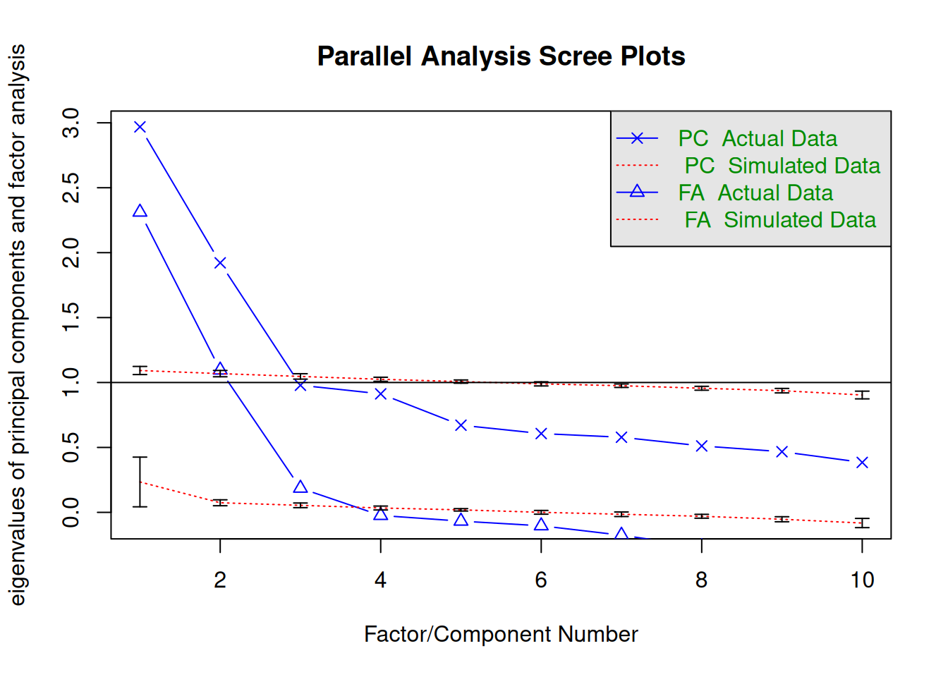
Parallel analysis suggests that the number of factors = 3 and the number of components = 2 Hull method
# Reduced correlation
HULL(select(bfi, O1:O5, A1:A5), eigen_type = "SMC")
ℹ Only CAF can be used as gof if method "PAF" is used. Setting gof to "CAF"ℹ 'x' was not a correlation matrix. Correlations are found from entered raw data.Hull Analysis performed testing 0 to 5 factors.
PAF estimation and the CAF fit index was used.
── Number of factors suggested by the Hull method ──────────────────────────────
◌ With CAF: 3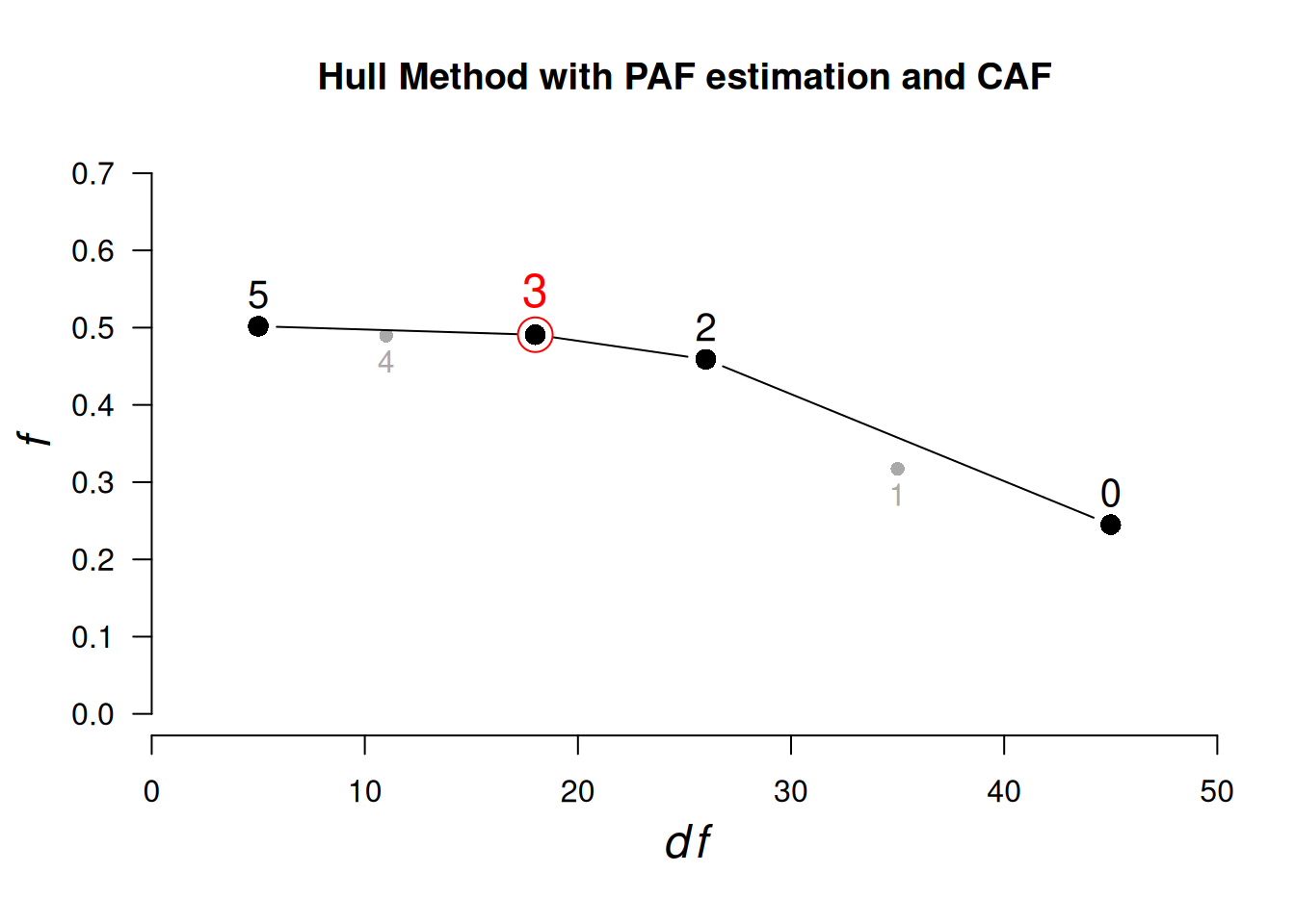
# Full correlation
HULL(select(bfi, O1:O5, A1:A5), eigen_type = "PCA")
ℹ Only CAF can be used as gof if method "PAF" is used. Setting gof to "CAF"
ℹ 'x' was not a correlation matrix. Correlations are found from entered raw data.Hull Analysis performed testing 0 to 3 factors.
PAF estimation and the CAF fit index was used.
── Number of factors suggested by the Hull method ──────────────────────────────
◌ With CAF: 2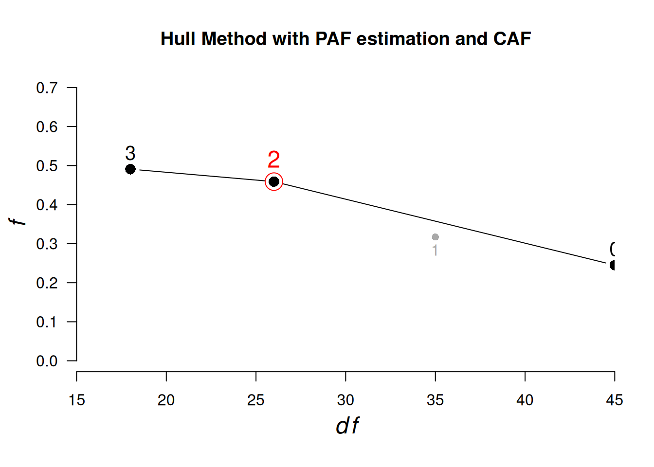
The conclusion is similar to parallel analysis.
Other methods
These should be examined as well. Note in this example, using fm = "pa" results in an error, so the suggestions are not based on PAF extraction.
psych::nfactors(select(bfi, O1:O5, A1:A5))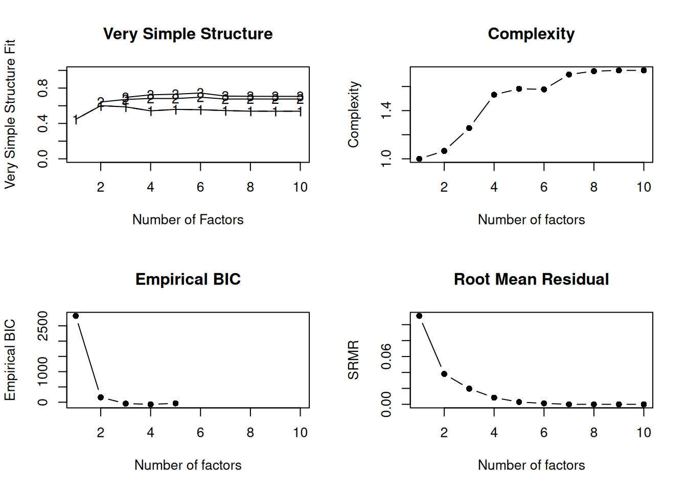
Number of factors
Call: vss(x = x, n = n, rotate = rotate, diagonal = diagonal, fm = fm,
    n.obs = n.obs, plot = FALSE, title = title, use = use, cor = cor)
VSS complexity 1 achieves a maximimum of 0.6  with  2  factors
VSS complexity 2 achieves a maximimum of 0.7  with  6  factors
The Velicer MAP achieves a minimum of 0.03  with  2  factors
Empirical BIC achieves a minimum of  -69.58  with  4  factors
Sample Size adjusted BIC achieves a minimum of  -27.76  with  4  factors

Statistics by number of factors
   vss1 vss2   map dof   chisq     prob sqresid  fit RMSEA  BIC  SABIC complex
1  0.45 0.00 0.036  35 1.6e+03 1.3e-311     7.9 0.45 0.126 1310 1421.4     1.0
2  0.60 0.64 0.032  26 3.2e+02  5.4e-53     5.1 0.64 0.064  117  199.1     1.1
3  0.59 0.67 0.052  18 9.5e+01  1.7e-12     4.3 0.69 0.039  -48    9.4     1.3
4  0.54 0.68 0.087  11 2.5e+01  1.0e-02     3.9 0.73 0.021  -63  -27.8     1.5
5  0.56 0.68 0.134   5 2.8e+00  7.2e-01     3.7 0.74 0.000  -37  -21.0     1.6
6  0.56 0.70 0.213   0 5.5e-01       NA     3.4 0.76    NA   NA     NA     1.6
7  0.55 0.68 0.314  -4 1.6e-07       NA     3.5 0.76    NA   NA     NA     1.7
8  0.54 0.68 0.650  -7 2.2e-07       NA     3.5 0.75    NA   NA     NA     1.7
9  0.54 0.68 1.000  -9 0.0e+00       NA     3.5 0.75    NA   NA     NA     1.7
10 0.54 0.68    NA -10 0.0e+00       NA     3.5 0.75    NA   NA     NA     1.7
    eChisq    SRMR  eCRMS eBIC
1  3.1e+03 1.1e-01 0.1259 2827
2  3.7e+02 3.8e-02 0.0502  160
3  9.8e+01 2.0e-02 0.0312  -45
4  1.8e+01 8.4e-03 0.0170  -70
5  2.1e+00 2.9e-03 0.0086  -38
6  3.7e-01 1.2e-03     NA   NA
7  1.2e-07 6.8e-07     NA   NA
8  1.4e-07 7.5e-07     NA   NA
9  1.1e-14 2.1e-10     NA   NA
10 1.1e-14 2.1e-10     NA   NA
Based on theoretical consideration, two factors seem reasonable.
Rotation
Complexity
Caution
The computation of variable complexity and factor complexity here are just for demonstrative purpose. You should not choose a rotation method based on these, because different rotations have different goals and complexity functions.
Unrotated solution
plot(fa_unrotated, labels = c(paste0("O", 1:5), paste0("A", 1:5)))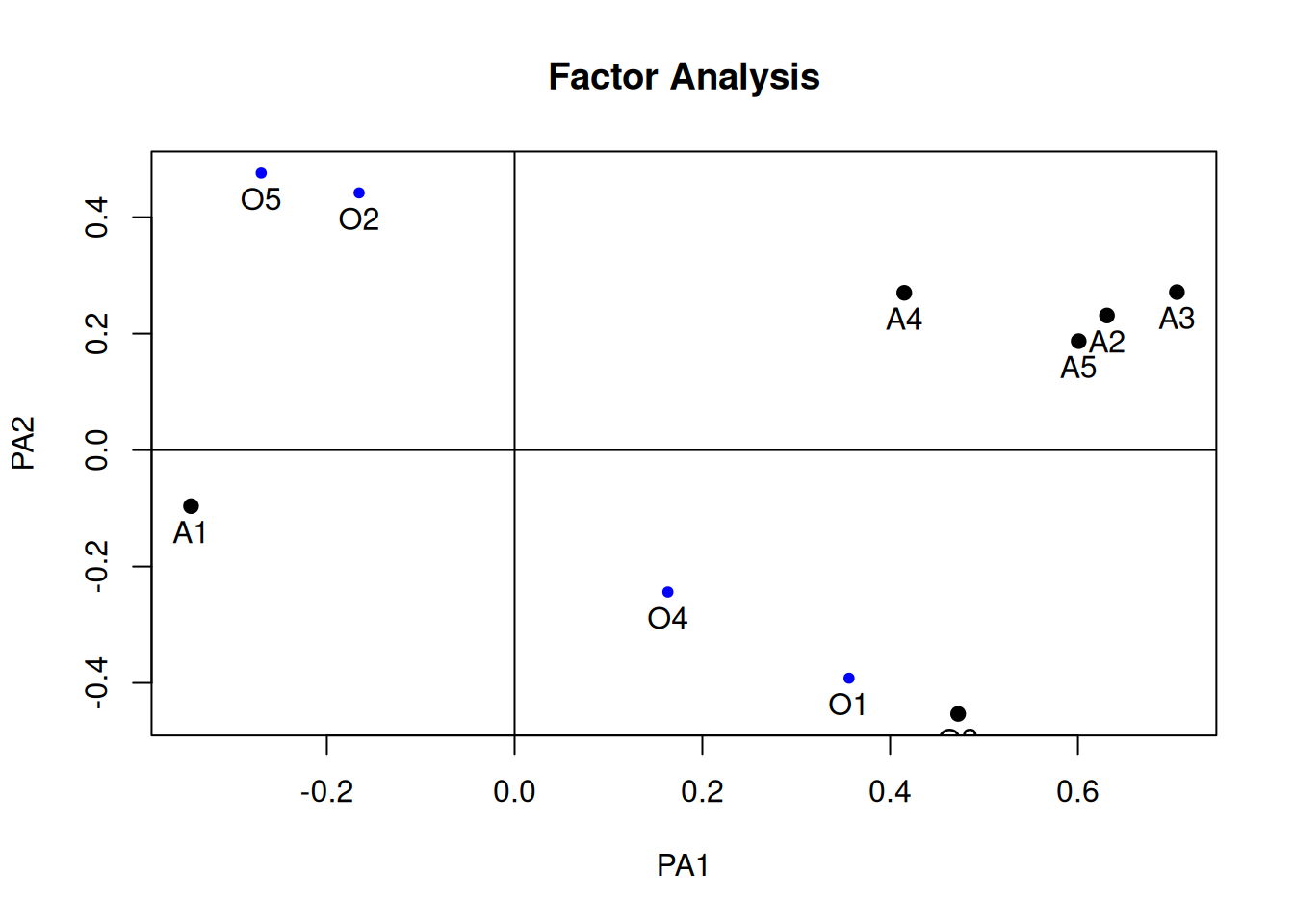
# Variable Complexity
lambda_unrotated <- fa_unrotated$loadings
sum(lambda_unrotated[, 1]^2 * lambda_unrotated[, 2]^2)
[1] 0.172905# Factor Complexity
fac_complexity <- 0
for (j in seq_len(ncol(lambda_unrotated))) {
for (i in seq_len(nrow(lambda_unrotated))) {
fac_complexity <- fac_complexity + sum(lambda_unrotated[i, j]^2 * lambda_unrotated[-i, j]^2)
}
}
fac_complexity[1] 4.447726Varimax
fa_varimax <- psych::fa(
    select(bfi, O1:O5, A1:A5),
    nfactors = 2, fm = "pa", rotate = "varimax")
plot(fa_varimax, labels = c(paste0("O", 1:5), paste0("A", 1:5)))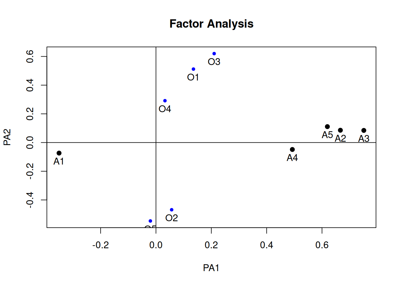
# Variable Complexity
(lambda_varimax <- fa_varimax$loadings)
Loadings:
   PA1    PA2
O1  0.135  0.512
O2        -0.468
O3  0.210  0.620
O4         0.292
O5        -0.546
A1 -0.350
A2  0.666
A3  0.751
A4  0.493
A5  0.619  0.111

                 PA1   PA2
SS loadings    1.825 1.284
Proportion Var 0.182 0.128
Cumulative Var 0.182 0.311sum(lambda_varimax[, 1]^2 * lambda_varimax[, 2]^2)[1] 0.03597018# Factor Complexity
fac_complexity <- 0
for (j in seq_len(ncol(lambda_varimax))) {
for (i in seq_len(nrow(lambda_varimax))) {
fac_complexity <- fac_complexity + sum(lambda_varimax[i, j]^2 * lambda_varimax[-i, j]^2)
}
}
fac_complexity[1] 3.877532Oblimin
fa_oblimin <- psych::fa(
    select(bfi, O1:O5, A1:A5),
    nfactors = 2, fm = "pa", rotate = "oblimin")
Loading required namespace: GPArotationplot(fa_oblimin, labels = c(paste0("O", 1:5), paste0("A", 1:5)))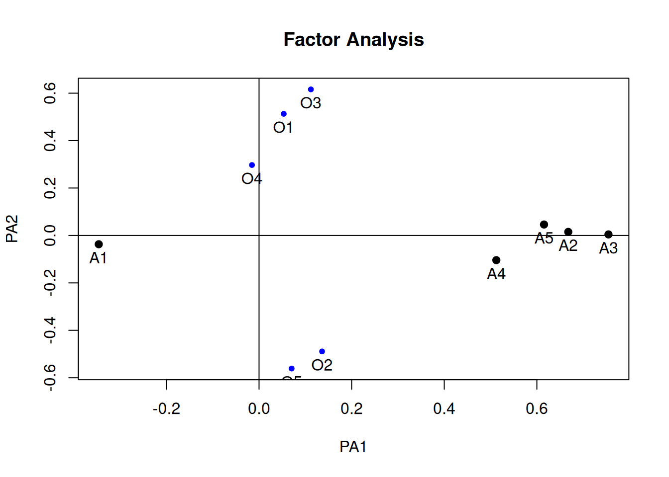
# Variable Complexity
(lambda_oblimin <- fa_oblimin$loadings)
Loadings:
   PA1    PA2
O1         0.513
O2  0.136 -0.489
O3  0.112  0.616
O4         0.297
O5        -0.561
A1 -0.346
A2  0.668
A3  0.755
A4  0.512 -0.104
A5  0.615

                 PA1   PA2
SS loadings    1.816 1.300
Proportion Var 0.182 0.130
Cumulative Var 0.182 0.312sum(lambda_oblimin[, 1]^2 * lambda_oblimin[, 2]^2)[1] 0.01545015# Factor Complexity
fac_complexity <- 0
for (j in seq_len(ncol(lambda_oblimin))) {
for (i in seq_len(nrow(lambda_oblimin))) {
fac_complexity <- fac_complexity + sum(lambda_oblimin[i, j]^2 * lambda_oblimin[-i, j]^2)
}
}
fac_complexity[1] 3.858235Geomin (Oblique)
fa_geomin <- psych::fa(
    select(bfi, O1:O5, A1:A5),
    nfactors = 2, fm = "pa", rotate = "geominQ")
plot(fa_geomin, labels = c(paste0("O", 1:5), paste0("A", 1:5)))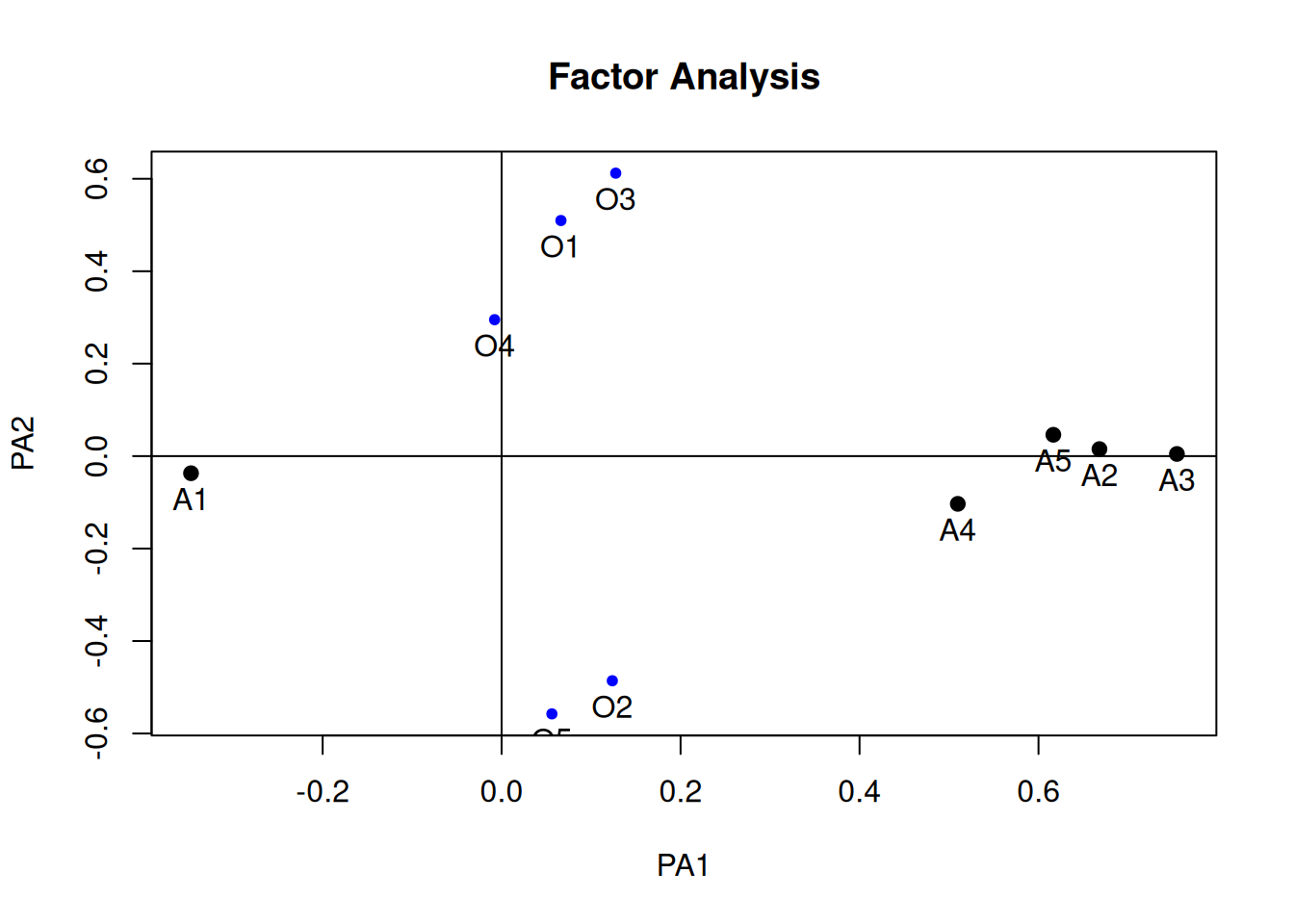
# Variable Complexity
(lambda_geomin <- fa_geomin$loadings)
Loadings:
   PA1    PA2
O1         0.510
O2  0.124 -0.486
O3  0.128  0.612
O4         0.295
O5        -0.558
A1 -0.347
A2  0.668
A3  0.755
A4  0.510 -0.103
A5  0.617

                 PA1   PA2
SS loadings    1.816 1.283
Proportion Var 0.182 0.128
Cumulative Var 0.182 0.310sum(lambda_geomin[, 1]^2 * lambda_geomin[, 2]^2)[1] 0.01569736# Factor Complexity
fac_complexity <- 0
for (j in seq_len(ncol(lambda_geomin))) {
for (i in seq_len(nrow(lambda_geomin))) {
fac_complexity <- fac_complexity + sum(lambda_geomin[i, j]^2 * lambda_geomin[-i, j]^2)
}
}
fac_complexity[1] 3.823991Target Rotation
In practice, we usually have some idea about the factor structure, and we can rotate the loadings to something close to that idea. This is an example of blurring the distinction between EFA and CFA.
Let’s say we think that the five O items are for one factor, and the five A items are for another.
# We want the first five items to load on factor 1 but not on factor 2,
# and the reverse for the next five items
target_mat <- matrix(
    c(NA, NA, NA, NA, NA, 0, 0, 0, 0, 0,
      0, 0, 0, 0, 0, NA, NA, NA, NA, NA),
    nrow = 10
)
fa_target <- psych::fa(
    select(bfi, O1:O5, A1:A5),
    nfactors = 2, fm = "pa",
    rotate = "targetQ", Target = target_mat)
fa_target
Factor Analysis using method = pa
Call: psych::fa(r = select(bfi, O1:O5, A1:A5), nfactors = 2, rotate = "targetQ",
fm = "pa", Target = target_mat)
Standardized loadings (pattern matrix) based upon correlation matrix
PA2 PA1 h2 u2 com
O1 0.06 0.51 0.280 0.72 1.0
O2 0.13 -0.49 0.223 0.78 1.1
O3 0.12 0.61 0.428 0.57 1.1
O4 -0.01 0.30 0.086 0.91 1.0
O5 0.06 -0.56 0.299 0.70 1.0
A1 -0.35 -0.04 0.128 0.87 1.0
A2 0.67 0.02 0.451 0.55 1.0
A3 0.75 0.01 0.571 0.43 1.0
A4 0.51 -0.10 0.245 0.75 1.1
A5 0.62 0.05 0.396 0.60 1.0
PA2 PA1
SS loadings 1.81 1.29
Proportion Var 0.18 0.13
Cumulative Var 0.18 0.31
Proportion Explained 0.58 0.42
Cumulative Proportion 0.58 1.00
With factor correlations of
PA2 PA1
PA2 1.00 0.25
PA1 0.25 1.00
Mean item complexity = 1
Test of the hypothesis that 2 factors are sufficient.
df null model = 45 with the objective function = 1.58 with Chi Square = 4409.68
df of the model are 26 and the objective function was 0.12
The root mean square of the residuals (RMSR) is 0.04
The df corrected root mean square of the residuals is 0.05
The harmonic n.obs is 2766 with the empirical chi square 362.29 with prob < 6e-61
The total n.obs was 2800 with Likelihood Chi Square = 323 with prob < 5.2e-53
Tucker Lewis Index of factoring reliability = 0.882
RMSEA index = 0.064 and the 90 % confidence intervals are 0.058 0.07
BIC = 116.63
Fit based upon off diagonal values = 0.97
Measures of factor score adequacy
PA2 PA1
Correlation of (regression) scores with factors 0.88 0.81
Multiple R square of scores with factors 0.77 0.66
Minimum correlation of possible factor scores 0.54 0.32Percentage of Variance Accounted For
Let’s use oblimin solution
# Proportion of variance by the first two eigenvalues
ev_oa <- fa_oblimin$e.values
sum(ev_oa[1:2]) / sum(ev_oa)
[1] 0.4399516The first two eigenvalues account for 44% of the total variance in the data.
Correlation Residual
This does not depend on rotation method.
round(fa_unrotated$residual, digits = 2) O1 O2 O3 O4 O5 A1 A2 A3 A4 A5
O1 0.72 0.02 0.05 0.02 0.04 0.10 0.00 0.00 0.02 0.02
O2 0.02 0.78 0.02 0.07 0.07 0.06 0.02 0.00 -0.01 0.02
O3 0.05 0.02 0.57 0.01 0.03 0.06 -0.03 0.01 0.00 0.04
O4 0.02 0.07 0.01 0.91 -0.02 -0.04 0.04 -0.01 -0.04 -0.04
O5 0.04 0.07 0.03 -0.02 0.70 0.07 -0.03 0.01 0.00 0.02
A1 0.10 0.06 0.06 -0.04 0.07 0.87 -0.10 0.00 0.02 0.04
A2 0.00 0.02 -0.03 0.04 -0.03 -0.10 0.55 -0.02 0.01 -0.03
A3 0.00 0.00 0.01 -0.01 0.01 0.00 -0.02 0.43 -0.01 0.03
A4 0.02 -0.01 0.00 -0.04 0.00 0.02 0.01 -0.01 0.75 0.01
A5 0.02 0.02 0.04 -0.04 0.02 0.04 -0.03 0.03 0.01 0.60As a general rule of thumb, researchers should pay attention to residuals with absolute value > .10. In our case, there were a few values close to .10, but it doesn’t seem to be strong evidence that there may be an additional factor needed.
Confidence Intervals
The loadings in EFA are quite unstable, especially with rotation. We can obtain confidence intervals using bootstrap, which is available in psych::fa() by specifying
fa_oblimin_boot <- psych::fa(
    select(bfi, O1:O5, A1:A5),
    nfactors = 2,
    n.iter = 200, # number of bootstrap samples
    fm = "pa", rotate = "oblimin")
fa_oblimin_boot
Factor Analysis with confidence intervals using method = psych::fa(r = select(bfi, O1:O5, A1:A5), nfactors = 2, n.iter = 200,
rotate = "oblimin", fm = "pa")
Factor Analysis using method = pa
Call: psych::fa(r = select(bfi, O1:O5, A1:A5), nfactors = 2, n.iter = 200,
rotate = "oblimin", fm = "pa")
Standardized loadings (pattern matrix) based upon correlation matrix
PA1 PA2 h2 u2 com
O1 0.05 0.51 0.280 0.72 1.0
O2 0.14 -0.49 0.223 0.78 1.2
O3 0.11 0.62 0.428 0.57 1.1
O4 -0.02 0.30 0.086 0.91 1.0
O5 0.07 -0.56 0.299 0.70 1.0
A1 -0.35 -0.04 0.128 0.87 1.0
A2 0.67 0.01 0.451 0.55 1.0
A3 0.75 0.00 0.571 0.43 1.0
A4 0.51 -0.10 0.245 0.75 1.1
A5 0.62 0.05 0.396 0.60 1.0
PA1 PA2
SS loadings 1.81 1.30
Proportion Var 0.18 0.13
Cumulative Var 0.18 0.31
Proportion Explained 0.58 0.42
Cumulative Proportion 0.58 1.00
With factor correlations of
PA1 PA2
PA1 1.00 0.26
PA2 0.26 1.00
Mean item complexity = 1
Test of the hypothesis that 2 factors are sufficient.
df null model = 45 with the objective function = 1.58 with Chi Square = 4409.68
df of the model are 26 and the objective function was 0.12
The root mean square of the residuals (RMSR) is 0.04
The df corrected root mean square of the residuals is 0.05
The harmonic n.obs is 2766 with the empirical chi square 362.29 with prob < 6e-61
The total n.obs was 2800 with Likelihood Chi Square = 323 with prob < 5.2e-53
Tucker Lewis Index of factoring reliability = 0.882
RMSEA index = 0.064 and the 90 % confidence intervals are 0.058 0.07
BIC = 116.63
Fit based upon off diagonal values = 0.97
Measures of factor score adequacy
PA1 PA2
Correlation of (regression) scores with factors 0.88 0.81
Multiple R square of scores with factors 0.77 0.66
Minimum correlation of possible factor scores 0.54 0.33
Coefficients and bootstrapped confidence intervals
low PA1 upper low PA2 upper
O1 0.02 0.05 0.10 0.46 0.51 0.56
O2 0.09 0.14 0.18 -0.53 -0.49 -0.44
O3 0.08 0.11 0.16 0.57 0.62 0.67
O4 -0.06 -0.02 0.03 0.25 0.30 0.35
O5 0.03 0.07 0.12 -0.61 -0.56 -0.51
A1 -0.40 -0.35 -0.29 -0.09 -0.04 0.01
A2 0.63 0.67 0.71 -0.02 0.01 0.05
A3 0.72 0.75 0.79 -0.03 0.00 0.04
A4 0.47 0.51 0.55 -0.14 -0.10 -0.06
A5 0.58 0.62 0.66 0.01 0.05 0.08
Interfactor correlations and bootstrapped confidence intervals
lower estimate upper
PA1-PA2 0.2 0.26 0.32In practice, you should use more bootstrap samples (e.g., 1999). We can do the same for target rotation:
fa_target_boot <- psych::fa(
    select(bfi, O1:O5, A1:A5),
    nfactors = 2,
    n.iter = 200, # number of bootstrap samples
    fm = "pa",
    rotate = "targetQ", Target = target_mat)
fa_target_boot
Factor Analysis with confidence intervals using method = psych::fa(r = select(bfi, O1:O5, A1:A5), nfactors = 2, n.iter = 200,
rotate = "targetQ", fm = "pa", Target = target_mat)
Factor Analysis using method = pa
Call: psych::fa(r = select(bfi, O1:O5, A1:A5), nfactors = 2, n.iter = 200,
rotate = "targetQ", fm = "pa", Target = target_mat)
Standardized loadings (pattern matrix) based upon correlation matrix
PA2 PA1 h2 u2 com
O1 0.06 0.51 0.280 0.72 1.0
O2 0.13 -0.49 0.223 0.78 1.1
O3 0.12 0.61 0.428 0.57 1.1
O4 -0.01 0.30 0.086 0.91 1.0
O5 0.06 -0.56 0.299 0.70 1.0
A1 -0.35 -0.04 0.128 0.87 1.0
A2 0.67 0.02 0.451 0.55 1.0
A3 0.75 0.01 0.571 0.43 1.0
A4 0.51 -0.10 0.245 0.75 1.1
A5 0.62 0.05 0.396 0.60 1.0
PA2 PA1
SS loadings 1.81 1.29
Proportion Var 0.18 0.13
Cumulative Var 0.18 0.31
Proportion Explained 0.58 0.42
Cumulative Proportion 0.58 1.00
With factor correlations of
PA2 PA1
PA2 1.00 0.25
PA1 0.25 1.00
Mean item complexity = 1
Test of the hypothesis that 2 factors are sufficient.
df null model = 45 with the objective function = 1.58 with Chi Square = 4409.68
df of the model are 26 and the objective function was 0.12
The root mean square of the residuals (RMSR) is 0.04
The df corrected root mean square of the residuals is 0.05
The harmonic n.obs is 2766 with the empirical chi square 362.29 with prob < 6e-61
The total n.obs was 2800 with Likelihood Chi Square = 323 with prob < 5.2e-53
Tucker Lewis Index of factoring reliability = 0.882
RMSEA index = 0.064 and the 90 % confidence intervals are 0.058 0.07
BIC = 116.63
Fit based upon off diagonal values = 0.97
Measures of factor score adequacy
PA2 PA1
Correlation of (regression) scores with factors 0.88 0.81
Multiple R square of scores with factors 0.77 0.66
Minimum correlation of possible factor scores 0.54 0.32
Coefficients and bootstrapped confidence intervals
low PA2 upper low PA1 upper
O1 0.03 0.06 0.10 0.46 0.51 0.56
O2 0.09 0.13 0.17 -0.54 -0.49 -0.44
O3 0.08 0.12 0.16 0.57 0.61 0.66
O4 -0.06 -0.01 0.04 0.24 0.30 0.35
O5 0.02 0.06 0.10 -0.61 -0.56 -0.51
A1 -0.40 -0.35 -0.30 -0.09 -0.04 0.01
A2 0.63 0.67 0.70 -0.02 0.02 0.06
A3 0.72 0.75 0.79 -0.02 0.01 0.04
A4 0.47 0.51 0.55 -0.14 -0.10 -0.07
A5 0.58 0.62 0.66 0.01 0.05 0.09
Interfactor correlations and bootstrapped confidence intervals
lower estimate upper
PA2-PA1 0.19 0.25 0.3Full BFI
Target rotation with BFI, with polychoric correlation
pcorr_bfi <- lavaan::lavCor(select(bfi, A1:O5), ordered = TRUE)
n_pcorr_bfi <-
    select(bfi, A1:O5) |>
    drop_na() |>
    nrow()
# Parallel analysis
psych::fa.parallel(
    pcorr_bfi,
    n.obs = n_pcorr_bfi,
    fm = "pa",
    error.bars = TRUE
)
Parallel analysis suggests that the number of factors = 6 and the number of components = 5 # Other methods
nfactors(pcorr_bfi, n.obs = n_pcorr_bfi)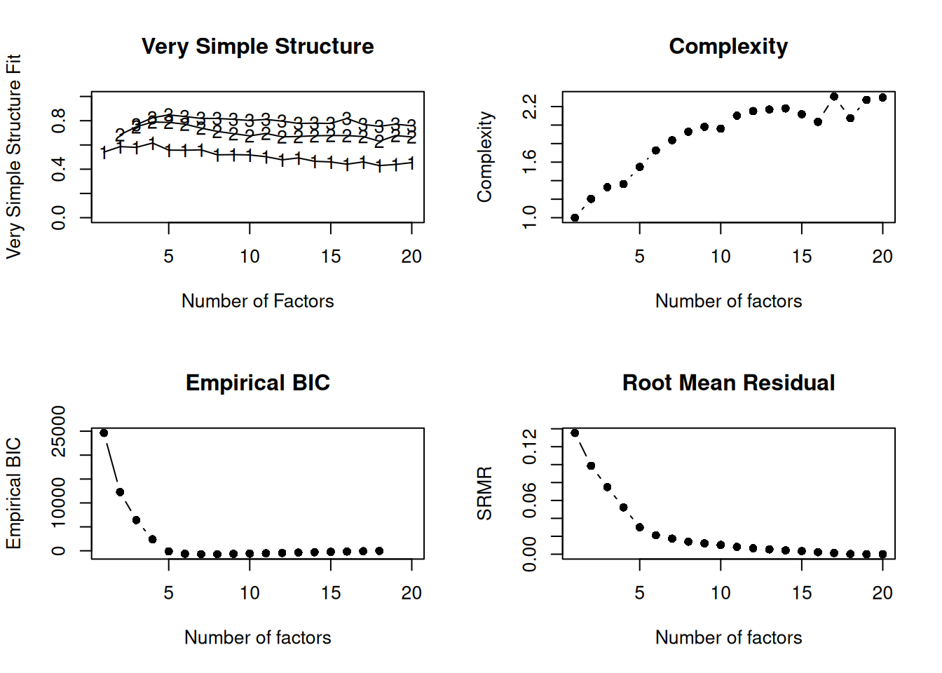
Number of factors
Call: vss(x = x, n = n, rotate = rotate, diagonal = diagonal, fm = fm,
    n.obs = n.obs, plot = FALSE, title = title, use = use, cor = cor)
VSS complexity 1 achieves a maximimum of Although the vss.max shows  4  factors, it is probably more reasonable to think about  2  factors
VSS complexity 2 achieves a maximimum of 0.79  with  4  factors
The Velicer MAP achieves a minimum of 0.02  with  5  factors
Empirical BIC achieves a minimum of  -711.98  with  8  factors
Sample Size adjusted BIC achieves a minimum of  -125.98  with  12  factors

Statistics by number of factors
   vss1 vss2   map dof   chisq     prob sqresid  fit  RMSEA   BIC   SABIC
1  0.54 0.00 0.032 275 1.4e+04  0.0e+00    27.3 0.54 0.1438 11980 12853.7
2  0.59 0.68 0.026 251 9.3e+03  0.0e+00    18.8 0.68 0.1213  7295  8092.2
3  0.58 0.75 0.023 228 6.6e+03  0.0e+00    13.9 0.77 0.1074  4860  5584.3
4  0.62 0.79 0.019 206 4.4e+03  0.0e+00    10.1 0.83 0.0912  2774  3428.8
5  0.56 0.79 0.016 185 2.2e+03  0.0e+00     7.6 0.87 0.0673   783  1370.9
6  0.56 0.77 0.017 165 1.4e+03 1.7e-188     6.6 0.89 0.0547    82   606.2
7  0.56 0.74 0.021 146 9.6e+02 1.8e-120     6.2 0.90 0.0479  -175   288.7
8  0.52 0.71 0.023 128 7.1e+02  1.2e-80     5.7 0.90 0.0430  -293   114.0
9  0.52 0.69 0.028 111 5.2e+02  5.4e-54     5.5 0.91 0.0388  -347     6.1
10 0.52 0.68 0.033  95 3.9e+02  1.0e-37     5.0 0.92 0.0358  -349   -47.0
11 0.50 0.70 0.040  80 2.5e+02  4.7e-20     5.0 0.92 0.0299  -369  -115.2
12 0.48 0.67 0.048  66 1.8e+02  2.3e-12     4.7 0.92 0.0265  -336  -126.0
13 0.49 0.67 0.058  53 1.3e+02  3.2e-08     4.5 0.92 0.0242  -285  -116.3
14 0.47 0.68 0.066  41 9.0e+01  1.8e-05     4.2 0.93 0.0220  -230   -99.9
15 0.46 0.68 0.081  30 6.0e+01  9.3e-04     3.7 0.94 0.0202  -174   -78.7
16 0.44 0.68 0.097  20 2.4e+01  2.5e-01     3.3 0.94 0.0089  -132   -68.5
17 0.46 0.67 0.114  11 7.8e+00  7.3e-01     3.7 0.94 0.0000   -78   -43.0
18 0.43 0.63 0.134   3 4.5e-01  9.3e-01     3.5 0.94 0.0000   -23   -13.4
19 0.44 0.68 0.157  -4 3.8e-04       NA     3.7 0.94     NA    NA      NA
20 0.45 0.67 0.199 -10 8.4e-05       NA     3.7 0.94     NA    NA      NA
   complex  eChisq    SRMR  eCRMS  eBIC
1      1.0 2.7e+04 1.4e-01 0.1414 24627
2      1.2 1.4e+04 9.9e-02 0.1078 12266
3      1.3 8.2e+03 7.5e-02 0.0859  6414
4      1.4 4.0e+03 5.2e-02 0.0631  2392
5      1.5 1.3e+03 3.0e-02 0.0383  -121
6      1.7 6.6e+02 2.1e-02 0.0286  -631
7      1.8 4.4e+02 1.7e-02 0.0249  -697
8      1.9 2.9e+02 1.4e-02 0.0214  -712
9      2.0 2.1e+02 1.2e-02 0.0198  -653
10     2.0 1.6e+02 1.0e-02 0.0184  -585
11     2.1 9.7e+01 8.2e-03 0.0158  -526
12     2.2 6.4e+01 6.6e-03 0.0141  -451
13     2.2 4.3e+01 5.4e-03 0.0129  -370
14     2.2 2.7e+01 4.3e-03 0.0117  -292
15     2.1 1.7e+01 3.5e-03 0.0109  -216
16     2.0 7.6e+00 2.3e-03 0.0088  -148
17     2.3 2.6e+00 1.3e-03 0.0070   -83
18     2.1 1.0e-01 2.6e-04 0.0026   -23
19     2.3 7.5e-05 7.2e-06     NA    NA
20     2.3 1.8e-05 3.5e-06     NA    NA
# Target rotation
target_mat_bfi <- matrix(0, nrow = 25, ncol = 5)
target_mat_bfi[1:5, 1] <- NA
target_mat_bfi[6:10, 2] <- NA
target_mat_bfi[11:15, 3] <- NA
target_mat_bfi[16:20, 4] <- NA
target_mat_bfi[21:25, 5] <- NA
fa_target_bfi <- psych::fa(
pcorr_bfi, n.obs = n_pcorr_bfi,
nfactors = 5, fm = "pa",
rotate = "targetQ", Target = target_mat_bfi)
fa_target_bfiFactor Analysis using method = pa
Call: psych::fa(r = pcorr_bfi, nfactors = 5, n.obs = n_pcorr_bfi, rotate = "targetQ",
fm = "pa", Target = target_mat_bfi)
Standardized loadings (pattern matrix) based upon correlation matrix
PA4 PA3 PA2 PA1 PA5 h2 u2 com
A1 0.15 0.18 0.07 -0.51 -0.09 0.26 0.74 1.5
A2 0.03 0.05 0.07 0.69 0.03 0.54 0.46 1.0
A3 0.02 0.18 0.02 0.69 0.04 0.61 0.39 1.1
A4 -0.02 0.10 0.21 0.47 -0.18 0.35 0.65 1.9
A5 -0.11 0.28 0.00 0.55 0.04 0.53 0.47 1.6
C1 0.07 -0.02 0.59 0.00 0.17 0.40 0.60 1.2
C2 0.18 -0.05 0.71 0.06 0.06 0.51 0.49 1.2
C3 0.04 -0.08 0.61 0.10 -0.07 0.36 0.64 1.1
C4 0.17 0.03 -0.69 0.01 -0.03 0.55 0.45 1.1
C5 0.21 -0.10 -0.60 0.01 0.12 0.49 0.51 1.4
E1 -0.01 -0.62 0.13 -0.07 -0.02 0.39 0.61 1.1
E2 0.17 -0.71 -0.01 -0.04 0.01 0.61 0.39 1.1
E3 0.07 0.51 -0.02 0.22 0.27 0.50 0.50 2.0
E4 -0.05 0.64 0.00 0.27 -0.13 0.60 0.40 1.4
E5 0.13 0.50 0.28 0.01 0.17 0.46 0.54 2.0
N1 0.86 0.21 0.01 -0.19 -0.08 0.74 0.26 1.2
N2 0.81 0.14 0.02 -0.16 0.00 0.66 0.34 1.1
N3 0.77 0.00 -0.03 0.02 0.01 0.59 0.41 1.0
N4 0.56 -0.33 -0.13 0.08 0.13 0.55 0.45 1.9
N5 0.56 -0.17 0.00 0.20 -0.15 0.40 0.60 1.6
O1 0.00 0.18 0.06 0.00 0.55 0.39 0.61 1.3
O2 0.20 0.02 -0.08 0.15 -0.50 0.30 0.70 1.6
O3 0.02 0.27 -0.01 0.05 0.63 0.54 0.46 1.4
O4 0.19 -0.28 -0.04 0.19 0.48 0.35 0.65 2.4
O5 0.11 0.05 -0.04 0.04 -0.59 0.36 0.64 1.1
PA4 PA3 PA2 PA1 PA5
SS loadings 2.96 2.61 2.33 2.26 1.85
Proportion Var 0.12 0.10 0.09 0.09 0.07
Cumulative Var 0.12 0.22 0.32 0.41 0.48
Proportion Explained 0.25 0.22 0.19 0.19 0.15
Cumulative Proportion 0.25 0.46 0.66 0.85 1.00
With factor correlations of
PA4 PA3 PA2 PA1 PA5
PA4 1.00 -0.21 -0.21 -0.09 0.02
PA3 -0.21 1.00 0.29 0.34 0.16
PA2 -0.21 0.29 1.00 0.23 0.20
PA1 -0.09 0.34 0.23 1.00 0.16
PA5 0.02 0.16 0.20 0.16 1.00
Mean item complexity = 1.4
Test of the hypothesis that 5 factors are sufficient.
df null model = 300 with the objective function = 9.59 with Chi Square = 23261.83
df of the model are 185 and the objective function was 0.92
The root mean square of the residuals (RMSR) is 0.03
The df corrected root mean square of the residuals is 0.04
The harmonic n.obs is 2436 with the empirical chi square 1322.13 with prob < 8.1e-171
The total n.obs was 2436 with Likelihood Chi Square = 2226.01 with prob < 0
Tucker Lewis Index of factoring reliability = 0.856
RMSEA index = 0.067 and the 90 % confidence intervals are 0.065 0.07
BIC = 783.36
Fit based upon off diagonal values = 0.98
Measures of factor score adequacy
PA4 PA3 PA2 PA1 PA5
Correlation of (regression) scores with factors 0.94 0.92 0.90 0.90 0.87
Multiple R square of scores with factors 0.89 0.84 0.81 0.81 0.76
Minimum correlation of possible factor scores 0.77 0.68 0.63 0.62 0.52Using the lavaan R package
More information at https://lavaan.ugent.be/tutorial/efa.html
# One- to Six-factor models
efa_fit <- efa(
    select(bfi, A1:O5),
    nfactors = 1:6,
    ordered = TRUE  # only needed for ordinal data
)
summary(efa_fit)
This is lavaan 0.6-19 -- running exploratory factor analysis
Estimator DWLS
Rotation method GEOMIN OBLIQUE
Geomin epsilon 0.001
Rotation algorithm (rstarts) GPA (30)
Standardized metric TRUE
Row weights None
Used Total
Number of observations 2436 2800
Overview models:
chisq df pvalue cfi rmsea
nfactors = 1 16233.810 275 0 0.363 0.148
nfactors = 2 10653.913 251 0 0.609 0.122
nfactors = 3 7391.517 228 0 0.723 0.107
nfactors = 4 4711.331 206 0 0.819 0.091
nfactors = 5 1856.317 185 0 0.914 0.066
nfactors = 6 1058.461 165 0 0.950 0.054
Eigenvalues correlation matrix:
ev1 ev2 ev3 ev4 ev5 ev6 ev7 ev8 ev9 ev10
5.725 2.960 2.294 1.964 1.638 1.050 0.797 0.767 0.669 0.637
ev11 ev12 ev13 ev14 ev15 ev16 ev17 ev18 ev19 ev20
0.620 0.584 0.560 0.541 0.504 0.480 0.453 0.429 0.413 0.383
ev21 ev22 ev23 ev24 ev25
0.354 0.335 0.328 0.310 0.203
Number of factors: 1
Standardized loadings: (* = significant at 1% level)
f1 unique.var communalities
A1 .* 0.930 0.070
A2 -0.503* 0.747 0.253
A3 -0.587* 0.655 0.345
A4 -0.432* 0.813 0.187
A5 -0.623* 0.611 0.389
C1 -0.377* 0.858 0.142
C2 -0.360* 0.871 0.129
C3 -0.330* 0.891 0.109
C4 0.510* 0.740 0.260
C5 0.510* 0.740 0.260
E1 0.418* 0.825 0.175
E2 0.626* 0.609 0.391
E3 -0.542* 0.706 0.294
E4 -0.624* 0.610 0.390
E5 -0.497* 0.753 0.247
N1 0.701* 0.508 0.492
N2 0.674* 0.546 0.454
N3 0.547* 0.700 0.300
N4 0.559* 0.688 0.312
N5 0.407* 0.834 0.166
O1 -0.355* 0.874 0.126
O2 .* 0.947 0.053
O3 -0.412* 0.830 0.170
O4 * 0.997 0.003
O5 .* 0.947 0.053
f1
Sum of squared loadings 5.769
Proportion of total 1.000
Proportion var 0.231
Cumulative var 0.231
Number of factors: 2
Standardized loadings: (* = significant at 1% level)
f1 f2 unique.var communalities
A1 .* * 0.925 0.075
A2 0.591* 0.656 0.344
A3 0.672* 0.554 0.446
A4 0.441* * 0.784 0.216
A5 0.641* .* 0.558 0.442
C1 0.431* 0.811 0.189
C2 0.451* 0.800 0.200
C3 0.338* * 0.869 0.131
C4 -0.420* .* 0.707 0.293
C5 -0.376* 0.343* 0.700 0.300
E1 -0.467* 0.776 0.224
E2 -0.579* .* 0.570 0.430
E3 0.663* * 0.571 0.429
E4 0.624* .* 0.563 0.437
E5 0.615* * 0.629 0.371
N1 0.859* 0.264 0.736
N2 0.845* 0.292 0.708
N3 0.750* 0.437 0.563
N4 .* 0.614* 0.539 0.461
N5 * 0.525* 0.705 0.295
O1 0.456* * 0.797 0.203
O2 .* * 0.944 0.056
O3 0.542* .* 0.713 0.287
O4 .* 0.304* 0.902 0.098
O5 .* 0.925 0.075
f1 f2 total
Sum of sq (obliq) loadings 4.821 3.188 8.009
Proportion of total 0.602 0.398 1.000
Proportion var 0.193 0.128 0.320
Cumulative var 0.193 0.320 0.320
Factor correlations: (* = significant at 1% level)
f1 f2
f1 1.000
f2 -0.161* 1.000
Number of factors: 3
Standardized loadings: (* = significant at 1% level)
f1 f2 f3 unique.var communalities
A1 .* * 0.902 0.098
A2 0.607* 0.615 0.385
A3 0.715* 0.483 0.517
A4 * 0.433* .* 0.767 0.233
A5 0.681* .* 0.496 0.504
C1 0.621* * 0.604 0.396
C2 0.648* 0.575 0.425
C3 0.474* .* 0.751 0.249
C4 -0.614* 0.371* 0.493 0.507
C5 -0.444* * 0.406* 0.608 0.392
E1 * -0.572* 0.685 0.315
E2 -0.619* .* 0.510 0.490
E3 .* 0.615* 0.548 0.452
E4 * 0.720* .* 0.451 0.549
E5 0.340* 0.442* 0.611 0.389
N1 0.859* 0.265 0.735
N2 * 0.840* 0.290 0.710
N3 0.751* 0.438 0.562
N4 .* 0.625* 0.533 0.467
N5 * 0.538* 0.700 0.300
O1 0.400* .* 0.746 0.254
O2 -0.373* * .* 0.849 0.151
O3 0.386* 0.331* * 0.678 0.322
O4 .* .* 0.864 0.136
O5 -0.393* 0.841 0.159
f2 f3 f1 total
Sum of sq (obliq) loadings 3.814 3.322 2.561 9.697
Proportion of total 0.393 0.343 0.264 1.000
Proportion var 0.153 0.133 0.102 0.388
Cumulative var 0.153 0.285 0.388 0.388
Factor correlations: (* = significant at 1% level)
f1 f2 f3
f1 1.000
f2 0.256* 1.000
f3 -0.003 -0.143* 1.000
Number of factors: 4
Standardized loadings: (* = significant at 1% level)
f1 f2 f3 f4 unique.var communalities
A1 .* * 0.904 0.096
A2 .* 0.592* 0.592 0.408
A3 .* 0.702* 0.470 0.530
A4 .* 0.423* .* 0.670 0.330
A5 0.672* .* 0.495 0.505
C1 0.563* .* 0.593 0.407
C2 0.679* * .* 0.495 0.505
C3 0.592* 0.644 0.356
C4 -0.657* .* .* 0.447 0.553
C5 -0.569* * 0.307* 0.524 0.476
E1 .* -0.571* * 0.675 0.325
E2 -0.616* .* .* 0.506 0.494
E3 0.626* 0.326* 0.506 0.494
E4 0.715* .* 0.442 0.558
E5 .* 0.441* .* 0.610 0.390
N1 0.866* * 0.256 0.744
N2 0.843* 0.291 0.709
N3 0.751* 0.435 0.565
N4 .* .* 0.606* 0.526 0.474
N5 0.567* .* 0.651 0.349
O1 .* 0.571* 0.607 0.393
O2 .* -0.523* 0.689 0.311
O3 0.358* 0.648* 0.457 0.543
O4 .* 0.373* 0.792 0.208
O5 .* -0.580* 0.657 0.343
f2 f3 f1 f4 total
Sum of sq (obliq) loadings 3.747 3.187 2.240 1.893 11.066
Proportion of total 0.339 0.288 0.202 0.171 1.000
Proportion var 0.150 0.127 0.090 0.076 0.443
Cumulative var 0.150 0.277 0.367 0.443 0.443
Factor correlations: (* = significant at 1% level)
f1 f2 f3 f4
f1 1.000
f2 0.237* 1.000
f3 -0.090* -0.137* 1.000
f4 0.096* 0.006 0.057 1.000
Number of factors: 5
Standardized loadings: (* = significant at 1% level)
f1 f2 f3 f4 f5 unique.var communalities
A1 -0.472* .* 0.744 0.256
A2 0.466* * 0.565* .* 0.467 0.533
A3 0.440* 0.685* * 0.383 0.617
A4 .* .* 0.401* .* 0.643 0.357
A5 0.346* 0.677* 0.459 0.541
C1 0.578* .* 0.593 0.407
C2 0.687* .* .* 0.492 0.508
C3 0.592* 0.643 0.357
C4 -0.673* .* .* 0.449 0.551
C5 -0.585* * 0.318* 0.505 0.495
E1 .* .* -0.604* * 0.598 0.402
E2 .* -0.653* .* 0.391 0.609
E3 0.665* .* 0.500 0.500
E4 0.743* .* .* 0.391 0.609
E5 .* .* 0.477* .* 0.542 0.458
N1 -0.530* 0.787* * 0.193 0.807
N2 -0.471* 0.760* 0.284 0.716
N3 .* 0.756* 0.418 0.582
N4 .* .* 0.655* * 0.441 0.559
N5 0.603* .* 0.601 0.399
O1 .* 0.545* 0.609 0.391
O2 * .* -0.518* 0.689 0.311
O3 0.409* 0.610* 0.461 0.539
O4 .* 0.301* 0.435* 0.656 0.344
O5 * -0.584* 0.643 0.357
f3 f4 f2 f5 f1 total
Sum of sq (obliq) loadings 3.832 3.012 2.224 1.795 1.344 12.207
Proportion of total 0.314 0.247 0.182 0.147 0.110 1.000
Proportion var 0.153 0.120 0.089 0.072 0.054 0.488
Cumulative var 0.153 0.274 0.363 0.435 0.488 0.488
Factor correlations: (* = significant at 1% level)
f1 f2 f3 f4 f5
f1 1.000
f2 0.078 1.000
f3 -0.100 0.293* 1.000
f4 0.113 -0.050 -0.130* 1.000
f5 0.018 0.011 0.008 0.025 1.000
Number of factors: 6
Standardized loadings: (* = significant at 1% level)
f1 f2 f3 f4 f5 f6 unique.var
A1 -0.607* .* .* 0.605
A2 0.648* 0.336* .* 0.401
A3 0.504* 0.539* * 0.392
A4 0.314* .* .* .* 0.646
A5 .* 0.627* .* 0.432
C1 0.598* .* 0.583
C2 0.733* .* 0.444
C3 * 0.586* .* 0.648
C4 .* -0.649* .* .* 0.392* 0.348
C5 -0.552* 0.337* .* 0.515
E1 .* -0.548* -0.382* 0.553
E2 -0.621* .* .* 0.380
E3 0.728* .* .* 0.457
E4 0.759* .* .* 0.362
E5 .* 0.478* .* .* 0.544
N1 0.595* 0.756* * 0.198
N2 0.578* 0.700* 0.258
N3 .* 0.749* 0.412
N4 .* * .* 0.630* .* 0.436
N5 .* * 0.610* .* 0.595
O1 * 0.364* 0.534* 0.585
O2 0.313* -0.514* 0.661
O3 0.467* 0.607* 0.459
O4 .* .* .* 0.456* 0.655
O5 .* .* -0.610* 0.575
communalities
A1 0.395
A2 0.599
A3 0.608
A4 0.354
A5 0.568
C1 0.417
C2 0.556
C3 0.352
C4 0.652
C5 0.485
E1 0.447
E2 0.620
E3 0.543
E4 0.638
E5 0.456
N1 0.802
N2 0.742
N3 0.588
N4 0.564
N5 0.405
O1 0.415
O2 0.339
O3 0.541
O4 0.345
O5 0.425
f3 f5 f2 f6 f1 f4 total
Sum of sq (obliq) loadings 3.451 2.971 2.228 1.685 1.485 1.034 12.856
Proportion of total 0.268 0.231 0.173 0.131 0.116 0.080 1.000
Proportion var 0.138 0.119 0.089 0.067 0.059 0.041 0.514
Cumulative var 0.138 0.257 0.346 0.413 0.473 0.514 0.514
Factor correlations: (* = significant at 1% level)
f1 f2 f3 f4 f5 f6
f1 1.000
f2 0.177* 1.000
f3 0.145* 0.268* 1.000
f4 -0.092 0.034 -0.032 1.000
f5 -0.015 -0.110 -0.289* -0.121 1.000
f6 0.022 0.164* -0.089 0.121* 0.120* 1.000 With target rotation
# Target rotation (using the same matrix defined above)
efa5fac_fit <- efa(
    select(bfi, A1:O5),
    nfactors = 5,
    ordered = TRUE,
    rotation = "target",
    rotation.args = list(
        target = target_mat_bfi
    )
)
summary(efa5fac_fit)
This is lavaan 0.6-19 -- running exploratory factor analysis
Estimator DWLS
Rotation method PST OBLIQUE
Rotation algorithm (rstarts) GPA (30)
Standardized metric TRUE
Row weights None
Used Total
Number of observations 2436 2800
Fit measures:
chisq df pvalue cfi rmsea
nfactors = 5 1856.317 185 0 0.914 0.066
Eigenvalues correlation matrix:
ev1 ev2 ev3 ev4 ev5 ev6 ev7 ev8 ev9 ev10
5.725 2.960 2.294 1.964 1.638 1.050 0.797 0.767 0.669 0.637
ev11 ev12 ev13 ev14 ev15 ev16 ev17 ev18 ev19 ev20
0.620 0.584 0.560 0.541 0.504 0.480 0.453 0.429 0.413 0.383
ev21 ev22 ev23 ev24 ev25
0.354 0.335 0.328 0.310 0.203
Standardized loadings: (* = significant at 1% level)
f1 f2 f3 f4 f5 unique.var communalities
A1 -0.502* * .* .* * 0.744 0.256
A2 0.684* * * 0.467 0.533
A3 0.693* .* * 0.383 0.617
A4 0.467* .* .* .* 0.643 0.357
A5 0.552* .* .* 0.459 0.541
C1 0.595* * .* 0.593 0.407
C2 * 0.705* * .* * 0.492 0.508
C3 .* 0.606* * * * 0.643 0.357
C4 -0.692* .* 0.449 0.551
C5 -0.604* .* .* .* 0.505 0.495
E1 * .* -0.636* 0.598 0.402
E2 * -0.710* .* 0.391 0.609
E3 .* 0.497* * .* 0.500 0.500
E4 .* 0.648* * .* 0.391 0.609
E5 .* 0.488* .* .* 0.542 0.458
N1 .* .* 0.896* * 0.193 0.807
N2 .* .* 0.848* 0.284 0.716
N3 * * 0.749* 0.418 0.582
N4 * .* -0.341* 0.555* .* 0.441 0.559
N5 .* .* 0.548* .* 0.601 0.399
O1 * .* 0.550* 0.609 0.391
O2 .* * .* -0.508* 0.689 0.311
O3 * .* 0.630* 0.461 0.539
O4 .* .* .* 0.474* 0.656 0.344
O5 * .* -0.591* 0.643 0.357
f4 f3 f2 f1 f5 total
Sum of sq (obliq) loadings 3.029 2.650 2.368 2.293 1.868 12.207
Proportion of total 0.248 0.217 0.194 0.188 0.153 1.000
Proportion var 0.121 0.106 0.095 0.092 0.075 0.488
Cumulative var 0.121 0.227 0.322 0.414 0.488 0.488
Factor correlations: (* = significant at 1% level)
f1 f2 f3 f4 f5
f1 1.000
f2 0.216* 1.000
f3 0.318* 0.284* 1.000
f4 -0.087* -0.206* -0.213* 1.000
f5 0.163* 0.204* 0.148* 0.020 1.000 APA Table
Openness and Agreeableness
fa_oblimin$loadings |>
    unclass() |>
    as.data.frame() |>
    tibble::rownames_to_column() |>
    flextable::flextable() |>
    bold(i = ~ abs(PA1) >= .30, j = ~ PA1) |>
    bold(i = ~ abs(PA2) >= .30, j = ~ PA2) |>
    set_formatter(
        PA1 = rmlead0,
        PA2 = rmlead0
    ) |>
    set_header_labels(values = c("item", "1", "2")) |>
    add_header_row(values = c("", "Factor loading"), colwidths = c(1, 2)) |>
    align(i = 1, align = "center", part = "header")
Factor loading | ||
|---|---|---|
item | 1 | 2 |
O1 | .05 | .51 |
O2 | .14 | -.49 |
O3 | .11 | .62 |
O4 | -.02 | .30 |
O5 | .07 | -.56 |
A1 | -.35 | -.04 |
A2 | .67 | .01 |
A3 | .75 | .00 |
A4 | .51 | -.10 |
A5 | .62 | .05 |
25-item from IPIP
fa_target_bfi$loadings |>
    unclass() |>
    as.data.frame() |>
    tibble::rownames_to_column() |>
    flextable::flextable() |>
    bold(i = ~ abs(PA1) >= .30, j = ~ PA1) |>
    bold(i = ~ abs(PA2) >= .30, j = ~ PA2) |>
    bold(i = ~ abs(PA3) >= .30, j = ~ PA3) |>
    bold(i = ~ abs(PA4) >= .30, j = ~ PA4) |>
    bold(i = ~ abs(PA5) >= .30, j = ~ PA5) |>
    set_formatter(
        PA1 = rmlead0,
        PA2 = rmlead0,
        PA3 = rmlead0,
        PA4 = rmlead0,
        PA5 = rmlead0
    ) |>
    set_header_labels(values = c("item", "1", "2", "3", "4", "5")) |>
    add_header_row(values = c("", "Factor loading"), colwidths = c(1, 5)) |>
    align(i = 1, align = "center", part = "header")
Factor loading | |||||
|---|---|---|---|---|---|
item | 1 | 2 | 3 | 4 | 5 |
A1 | .15 | .18 | .07 | -.51 | -.09 |
A2 | .03 | .05 | .07 | .69 | .03 |
A3 | .02 | .18 | .02 | .69 | .04 |
A4 | -.02 | .10 | .21 | .47 | -.18 |
A5 | -.11 | .28 | -.00 | .55 | .04 |
C1 | .07 | -.02 | .59 | -.00 | .17 |
C2 | .18 | -.05 | .71 | .06 | .06 |
C3 | .04 | -.08 | .61 | .10 | -.07 |
C4 | .17 | .03 | -.69 | .01 | -.03 |
C5 | .21 | -.10 | -.60 | .01 | .12 |
E1 | -.01 | -.62 | .13 | -.07 | -.02 |
E2 | .17 | -.71 | -.01 | -.04 | .01 |
E3 | .07 | .51 | -.02 | .22 | .27 |
E4 | -.05 | .64 | -.00 | .27 | -.13 |
E5 | .13 | .50 | .28 | .01 | .17 |
N1 | .86 | .21 | .01 | -.19 | -.08 |
N2 | .81 | .14 | .02 | -.16 | .00 |
N3 | .77 | .00 | -.03 | .02 | .01 |
N4 | .56 | -.33 | -.13 | .08 | .13 |
N5 | .56 | -.17 | -.00 | .20 | -.15 |
O1 | -.00 | .18 | .06 | -.00 | .55 |
O2 | .20 | .02 | -.08 | .15 | -.50 |
O3 | .02 | .27 | -.01 | .05 | .63 |
O4 | .19 | -.28 | -.04 | .19 | .48 |
O5 | .11 | .05 | -.04 | .04 | -.59 |