# dput({set.seed(1421); sample(rep(25:36, c(3, 8, 7, 5, 5, 7, 3, 2, 2, 6, 2, 2)))})
raw_score <- c(26, 25, 33, 31, 26, 34, 29, 36, 25, 29, 28, 32, 25,
               30, 27, 31, 30, 30, 35, 30, 27, 26, 34, 32, 26, 34,
               30, 28, 28, 31, 30, 27, 26, 29, 29, 33, 27, 35, 26,
27, 28, 29, 28, 27, 34, 36, 26, 26, 34, 30, 34, 27)Norms and Standardized Scores
The following inputs raw scores from Table 2.1 of the text.
Frequency Distribution
The following recreates Table 2.1 using R.
freq <- table(raw_score)  # frequency
cumfreq <- cumsum(freq)  # cumulative frequency
perc <- prop.table(freq) * 100  # percentage
cumperc <- cumsum(perc)  # cumulative percentage
pr <- (cumperc - 0.5 * perc)  # percentile rank
cbind(freq, cumfreq, perc, cumperc, pr)
freq cumfreq perc cumperc pr
25 3 3 5.769231 5.769231 2.884615
26 8 11 15.384615 21.153846 13.461538
27 7 18 13.461538 34.615385 27.884615
28 5 23 9.615385 44.230769 39.423077
29 5 28 9.615385 53.846154 49.038462
30 7 35 13.461538 67.307692 60.576923
31 3 38 5.769231 73.076923 70.192308
32 2 40 3.846154 76.923077 75.000000
33 2 42 3.846154 80.769231 78.846154
34 6 48 11.538462 92.307692 86.538462
35 2 50 3.846154 96.153846 94.230769
36 2 52 3.846154 100.000000 98.076923Percentile Points
Score points for a particular percentile ranks
# P74
quantile(raw_score, .74)
74%
31.74 # Use a different type (see https://en.wikipedia.org/wiki/Quantile#Estimating_quantiles_from_a_sample)
quantile(raw_score, .74, type = 6)74%
32 Standardized Scores
\(z\)-score
z_score <- (raw_score - mean(raw_score)) / sd(raw_score)
c(mean = mean(z_score), sd = sd(z_score))
mean sd
-4.937123e-16 1.000000e+00 \(T\)-score
T_score <- z_score * 10 + 50
c(mean = mean(T_score), sd = sd(T_score))
mean sd
50 10
Important
Standardization does not change the shape of the distribution.
hist(raw_score)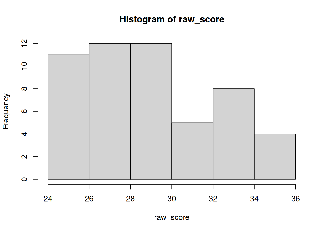
hist(z_score)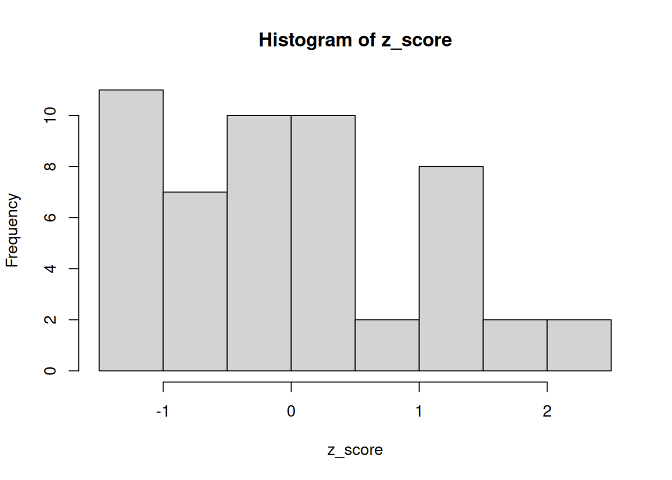
hist(T_score)
However, the histograms may look slightly different as each plot uses somewhat different ways to bin the values. But if you compute the skewness and the kurtosis, they should not be affected by the transformation.
Normalized Scores
Normalized \(z\)-score
# Using normal quantile
qnorm_pr <- qnorm(pr / 100)
# Convert raw scores
normalized_zscore <- as.vector(qnorm_pr[as.character(raw_score)])
hist(normalized_zscore)  # the shape will be closer to normal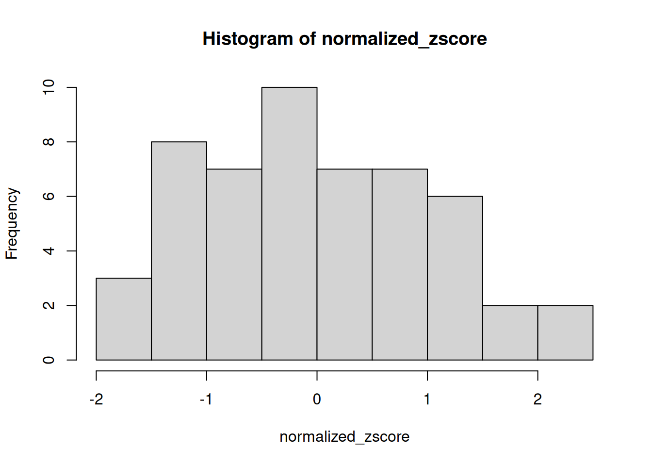
Age/Grade Equivalents
The following shows some fake data with two groups, one at age 5 and the other at age 6. The two groups took different forms of the test, and each form has 12 anchor/common items and 24 other items. The total score is the sum of the anchor and other items.
# Create data
y5 <- structure(c(14L, 12L, 18L, 8L, 12L, 20L, 16L, 18L, 11L, 21L,
11L, 20L, 18L, 14L, 20L, 13L, 11L, 17L, 19L, 16L, 18L, 14L, 14L,
19L, 18L, 4L, 4L, 12L, 8L, 28L, 18L, 12L, 16L, 9L, 10L, 18L,
12L, 12L, 21L, 15L, 22L, 12L, 8L, 11L, 18L, 10L, 14L, 14L, 5L,
8L, 11L, 16L, 11L, 13L, 10L, 12L, 8L, 18L, 18L, 15L, 17L, 19L,
21L, 15L, 22L, 12L, 15L, 15L, 22L, 20L, 11L, 15L, 16L, 13L, 17L,
17L, 19L, 11L, 13L, 15L, 15L, 12L, 16L, 12L, 15L, 16L, 18L, 15L,
21L, 21L, 18L, 7L, 15L, 18L, 18L, 16L, 16L, 18L, 17L, 19L, 5L,
2L, 8L, 2L, 2L, 4L, 3L, 7L, 5L, 7L, 6L, 6L, 6L, 4L, 8L, 3L, 3L,
3L, 2L, 6L, 4L, 4L, 4L, 5L, 7L, 1L, 1L, 3L, 5L, 8L, 5L, 3L, 5L,
3L, 4L, 6L, 4L, 4L, 5L, 4L, 6L, 2L, 4L, 2L, 3L, 6L, 4L, 3L, 0L,
1L, 3L, 5L, 3L, 6L, 2L, 1L, 2L, 5L, 7L, 6L, 5L, 5L, 8L, 3L, 5L,
3L, 3L, 3L, 6L, 4L, 5L, 5L, 4L, 4L, 6L, 2L, 7L, 3L, 6L, 4L, 4L,
4L, 6L, 3L, 6L, 6L, 7L, 3L, 6L, 6L, 4L, 0L, 4L, 5L, 4L, 6L, 4L,
5L, 6L, 6L), dim = c(100L, 2L), dimnames = list(NULL, c("total",
"anchor")))
y6 <- structure(c(20L, 15L, 10L, 12L, 20L, 14L, 13L, 15L, 24L, 22L,
15L, 16L, 21L, 24L, 9L, 19L, 12L, 13L, 14L, 18L, 10L, 23L, 19L,
11L, 12L, 13L, 18L, 21L, 22L, 22L, 24L, 16L, 13L, 4L, 17L, 24L,
12L, 14L, 23L, 12L, 20L, 16L, 20L, 15L, 12L, 20L, 14L, 8L, 24L,
5L, 26L, 23L, 12L, 15L, 18L, 19L, 18L, 11L, 16L, 17L, 18L, 16L,
19L, 18L, 17L, 17L, 20L, 10L, 12L, 14L, 18L, 10L, 16L, 21L, 15L,
14L, 9L, 13L, 18L, 15L, 4L, 19L, 16L, 21L, 14L, 15L, 26L, 23L,
21L, 20L, 17L, 13L, 10L, 15L, 13L, 21L, 17L, 18L, 24L, 18L, 5L,
5L, 3L, 6L, 7L, 6L, 4L, 5L, 5L, 8L, 4L, 7L, 8L, 7L, 5L, 8L, 3L,
4L, 5L, 6L, 3L, 9L, 6L, 5L, 4L, 3L, 5L, 7L, 8L, 8L, 6L, 5L, 6L,
2L, 5L, 6L, 4L, 6L, 8L, 3L, 7L, 4L, 6L, 5L, 5L, 9L, 7L, 2L, 9L,
2L, 9L, 8L, 3L, 5L, 8L, 6L, 7L, 3L, 6L, 6L, 5L, 6L, 8L, 6L, 8L,
6L, 10L, 6L, 2L, 6L, 6L, 5L, 8L, 8L, 8L, 8L, 3L, 5L, 7L, 5L,
0L, 7L, 7L, 9L, 4L, 5L, 6L, 7L, 6L, 7L, 8L, 6L, 1L, 2L, 5L, 6L,
6L, 7L, 10L, 6L), dim = c(100L, 2L), dimnames = list(NULL, c("total",
"anchor")))