ROC and MTMM

# Define a function for formatting numbers
comma <- function(x, d = 2) format(x, digits = d, big.mark = ",")

library(readxl)  # for reading excel data
library(haven)  # for reading SPSS data
library(ROCit)  # for ROC analysis
library(psych)
library(tidyverse)
library(modelsummary)  # for summarizing data

Classification Accuracy

Data analyzed in this paper: https://journals.sagepub.com/doi/10.1177/07342829211067128

tmp_path <- tempfile(fileext = "xlsx")  # temporary file
download.file("https://osf.io/download/tsm7x/", destfile = tmp_path)
dat1 <- readxl::read_xlsx(tmp_path, na = "NA")
dat1$asd <- recode(
    dat1$`Diagnosis(1=Non-typically developing; 2=ASD; 3=Neurotypical)`,
    `1` = "Non-TD",
    `2` = "ASD",
    `3` = "TD"
)
# Filter out Neurotypical
dat1_sub <- filter(dat1, asd != "TD")

First, sum the 16 items. Note that the sum is missing if any one item is missing

dat1_sub$ADEC <- rowSums(select(dat1_sub, ADEC_I01:ADEC_I16))  # NA if any item is NA
# Or treat missing as 0
dat1_sub$ADEC_rm_na <- rowSums(select(dat1_sub, ADEC_I01:ADEC_I16), na.rm = TRUE)

Now, we can look at the distribution of ADEC sum score by diagnosis:

ggplot(dat1_sub, aes(x = ADEC)) +
    geom_histogram() +
    facet_wrap(~ asd)

`stat_bin()` using `bins = 30`. Pick better value with `binwidth`.

Warning: Removed 12 rows containing non-finite values (`stat_bin()`).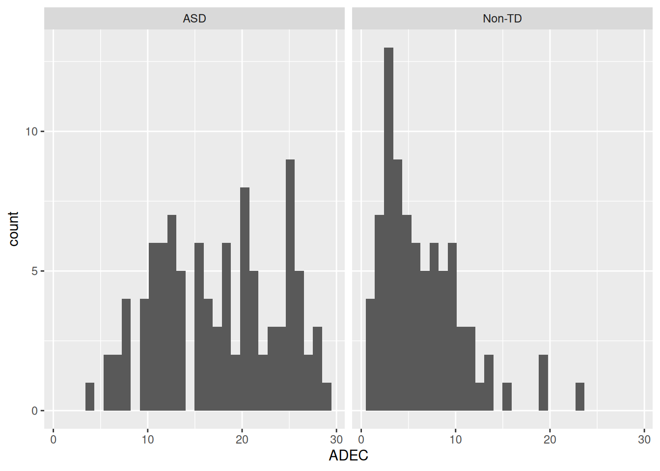

Classification Table

Let’s first use ADEC = 11 as cutoff. We then get the following contingency table

with(dat1_sub,
    table(ADEC >= 11, asd))

       asd
        ASD Non-TD
  FALSE  13     68
  TRUE   86     13

So the accuracy with this cutoff is (86 + 68) / 180 = 0.86. The sensitivity is 86 / (86 + 13) = 0.87, and the specificity is 68 / (68 + 13) = 0.84.

ROC

We can plot an ROC curve

compute_sens <- function(
    cut, x = dat1_sub$ADEC,
    crit = dat1_sub$asd == "ASD") {
    tp <- sum(x >= cut & crit, na.rm = TRUE)
    fn <- sum(x < cut & crit, na.rm = TRUE)
    tp / (tp + fn)
}
compute_spec <- function(
    cut, x = dat1_sub$ADEC,
    crit = dat1_sub$asd == "ASD") {
    tn <- sum(x < cut & !crit, na.rm = TRUE)
    fp <- sum(x >= cut & !crit, na.rm = TRUE)
    tn / (tn + fp)
}
sensitivity <- lapply(32:0, compute_sens) |>
    unlist()
specificity <- lapply(32:0, compute_spec) |>
    unlist()
data.frame(sensitivity, fpr = 1 - specificity) |>
    ggplot(aes(x = fpr, y = sensitivity)) +
    geom_point() +
    geom_line()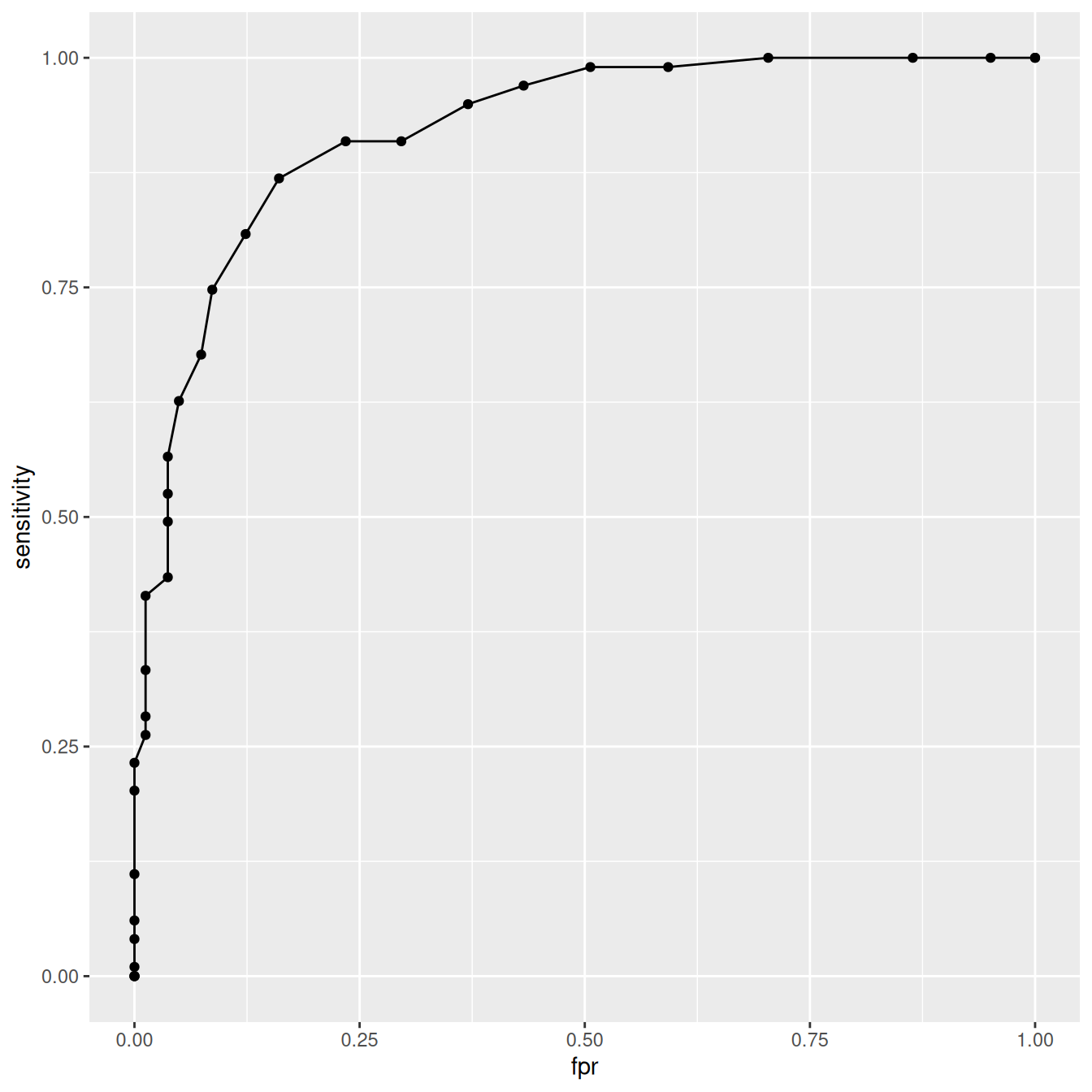

# AUC
dfpr <- c(diff(1 - specificity), 0)
dsens <- c(diff(sensitivity), 0)
sum(sensitivity * dfpr) + sum(dsens * dfpr) / 2

[1] 0.920626

Questions

Q1

Which cutoff gives the smallest difference between sensitivity and specificity? Please show your code.

# Your code and answer here

Q2

If one wants at least 90% sensitivity, what is the maximum specificity one can get?

Answer:

You can also use the ROCit package

roc_adec <- rocit(dat1_sub$ADEC, class = dat1_sub$asd == "ASD")

Warning in rocit(dat1_sub$ADEC, class = dat1_sub$asd == "ASD"): NA(s) in score
and/or class, removed from the data.

plot(roc_adec)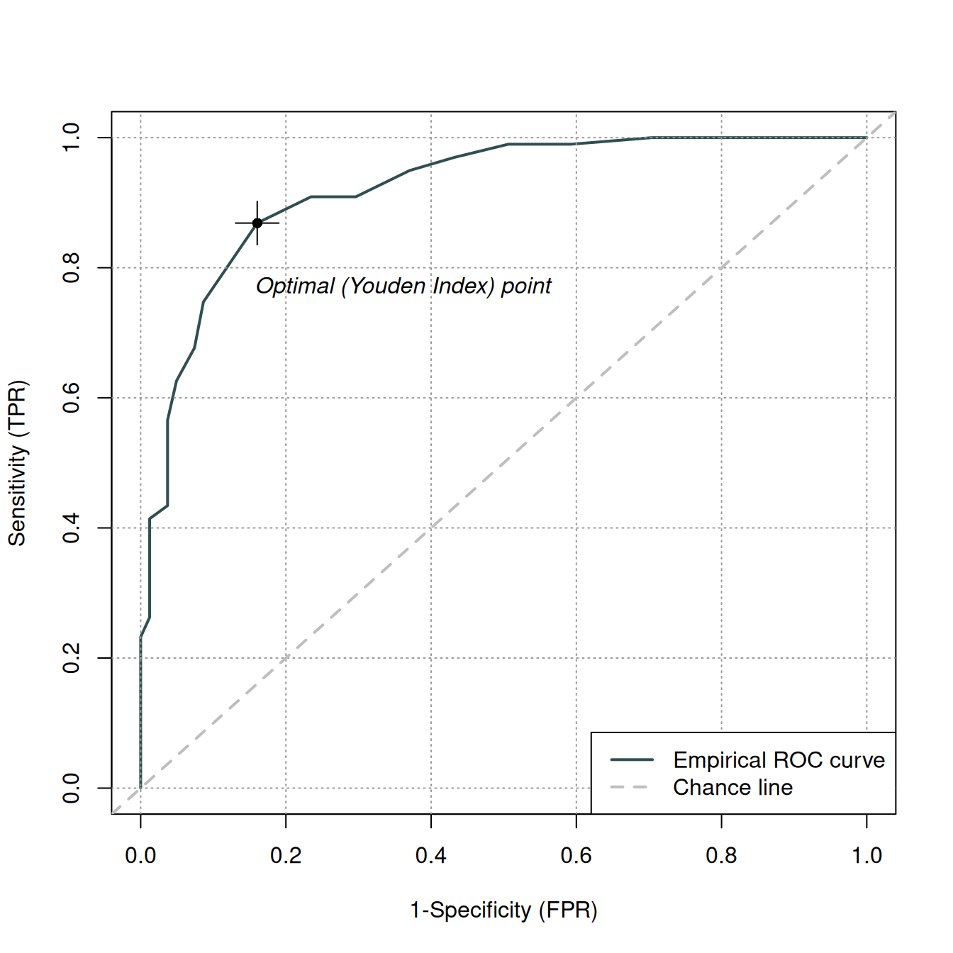

summary(roc_adec)

                          
 Method used: empirical   
 Number of positive(s): 99
 Number of negative(s): 81
 Area under curve: 0.9206 

ciAUC(roc_adec)

                                                          
   estimated AUC : 0.920626013218606                      
   AUC estimation method : empirical                      
                                                          
   CI of AUC                                              
   confidence level = 95%                                 
   lower = 0.880257283328194     upper = 0.960994743109017

Questions

The following shows the item discrimination values for the 16 items:

compute_discrimination <- function(i, data = dat1_sub[, 4:19]) {
    # Exclude Item i
    person_mean_noi <- rowMeans(data[, -i], na.rm = TRUE)
    # Correlation
    cor(data[[i]], person_mean_noi, use = "complete")
}
# Apply to all items
sapply(1:16, FUN = compute_discrimination) |> round(2)

 [1] 0.70 0.50 0.20 0.67 0.55 0.64 0.54 0.57 0.36 0.71 0.65 0.51 0.30 0.28 0.62
[16] 0.53

Q3

Repeat the ROC and AUC analysis, but using only the five items with the highest discrimination values.

# Your code and answer here

MTMM

Data from this paper: https://drive.google.com/file/d/1O4_MVWchC5kyCaf5p7GH4AjRIrY8zHJ8/

dat <- haven::read_sav("https://osf.io/download/5ayjb/")
dat_red <- haven::read_sav("https://osf.io/download/3uecq/")

The data set contains scale scores for Neuroticism (N), Extraversion (E), Openness (O), Agreeableness (A), and Conscientiousness (C) with four methods of assessment: Self-reports (SR), from a close-other who is a female (RF), from a close-other who is a male (RM), implicit association tests (IAT), and behavioral assessment (BIH). You can see the labels in the SPSS data set using

# Loop over each column, and call `attr(which = "label")` for each column
# to obtain the label stored as an attribute
dat_labels <- lapply(dat_red, FUN = attr, which = "label")
# Put things into a table (tibble format)
tibble(variable = names(dat_red), label = unlist(dat_labels))

# A tibble: 43 × 2
   variable label                              
   <chr>    <chr>                              
 1 age      age of respondent                  
 2 sex      sex                                
 3 NSR      Neoroticism-self report total      
 4 ESR      Extraversion-self report total     
 5 OSR      Openness-self report total         
 6 ASR      Agreeableness-self report total    
 7 CSR      Conscientiousness-self report total
 8 NRF      Neoroticism total-female rating    
 9 ERF      Extraversion total-female rating   
10 ORF      Openness total-female rating       
# ℹ 33 more rows

To make the size of the matrix a bit more manageable, we will select only E, A, and C for illustration, and with the SR, RF, and IAT methods.

Descriptive Statistics

Here are the descriptives:

var_names <- c("ESR", "ASR", "CSR", "ERF", "ARF", "CRF", "EIAT", "AIAT", "CIAT")
datasummary_skim(dat_red[var_names])

Warning in attr(x, "align"): 'xfun::attr()' is deprecated.
Use 'xfun::attr2()' instead.
See help("Deprecated")

	Unique (#)	Missing (%)	Mean	SD	Min	Median	Max
ESR	73	0	111.5	23.1	41.0	112.0	163.0
ASR	79	0	114.9	24.3	35.0	116.5	163.0
CSR	73	0	126.7	24.2	60.0	131.5	175.0
ERF	63	0	111.7	21.0	47.0	112.0	159.0
ARF	69	0	122.1	20.6	57.0	124.0	162.0
CRF	67	0	140.7	22.5	75.0	141.0	182.0
EIAT	146	0	0.2	0.4	−1.1	0.2	1.1
AIAT	146	0	0.5	0.4	−0.5	0.5	1.3
CIAT	146	0	0.5	0.4	−1.0	0.5	1.6

MTMM Matrix

datasummary_correlation(dat_red[var_names])

Warning in attr(x, "align"): 'xfun::attr()' is deprecated.
Use 'xfun::attr2()' instead.
See help("Deprecated")

	ESR	ASR	CSR	ERF	ARF	CRF	EIAT	AIAT	CIAT
ESR	1	.	.	.	.	.	.	.	.
ASR	.19	1	.	.	.	.	.	.	.
CSR	.20	.31	1	.	.	.	.	.	.
ERF	.60	.26	.08	1	.	.	.	.	.
ARF	.08	.57	.09	.24	1	.	.	.	.
CRF	.06	.17	.46	.28	.30	1	.	.	.
EIAT	.07	−.06	.10	.01	−.03	−.01	1	.	.
AIAT	−.03	−.12	−.05	−.19	−.03	.02	.11	1	.
CIAT	.01	.03	.08	−.12	.01	.06	.05	.28	1

Questions

Q4

Do the IAT measures show convergent validity with other measures? Report the relevant coefficients.

Answer: